US5280564A - Neural network having an optimized transfer function for each neuron - Google Patents

Neural network having an optimized transfer function for each neuron Download PDF

Info

Publication number
US5280564A
US5280564A US07/836,593 US83659392A US5280564A US 5280564 A US5280564 A US 5280564A US 83659392 A US83659392 A US 83659392A US 5280564 A US5280564 A US 5280564A
Authority
US
United States
Prior art keywords
data
function
neural network
weighting
layer
Prior art date
Legal status (The legal status is an assumption and is not a legal conclusion. Google has not performed a legal analysis and makes no representation as to the accuracy of the status listed.)
Expired - Fee Related
Application number
US07/836,593
Inventor
Kazuyuki Shiomi
Sei Watanabe
Current Assignee (The listed assignees may be inaccurate. Google has not performed a legal analysis and makes no representation or warranty as to the accuracy of the list.)
Honda Motor Co Ltd
Original Assignee
Honda Motor Co Ltd
Priority date (The priority date is an assumption and is not a legal conclusion. Google has not performed a legal analysis and makes no representation as to the accuracy of the date listed.)
Filing date
Publication date
Application filed by Honda Motor Co Ltd filed Critical Honda Motor Co Ltd
Assigned to HONDA GIKEN KOGYO KABUSHIKI KAISHA A COMPANY OF JAPAN reassignment HONDA GIKEN KOGYO KABUSHIKI KAISHA A COMPANY OF JAPAN ASSIGNMENT OF ASSIGNORS INTEREST. Assignors: SHIOMI, KAZUYUKI, WATANABE, SEI
Application granted granted Critical
Publication of US5280564A publication Critical patent/US5280564A/en
Anticipated expiration legal-status Critical
Expired - Fee Related legal-status Critical Current

Links

Images

Classifications

    • GPHYSICS
    • G06COMPUTING; CALCULATING OR COUNTING
    • G06NCOMPUTING ARRANGEMENTS BASED ON SPECIFIC COMPUTATIONAL MODELS
    • G06N3/00Computing arrangements based on biological models
    • G06N3/02Neural networks
    • G06N3/08Learning methods
    • GPHYSICS
    • G06COMPUTING; CALCULATING OR COUNTING
    • G06NCOMPUTING ARRANGEMENTS BASED ON SPECIFIC COMPUTATIONAL MODELS
    • G06N3/00Computing arrangements based on biological models
    • G06N3/02Neural networks
    • G06N3/04Architecture, e.g. interconnection topology
    • G06N3/048Activation functions

Definitions

  • the present invention is related to a neural network and particularly to a neural network which can learn with high precision and at a high speed.
  • Neural networks which perform signal operations in parallel using neurons that process signals in a similar manner to neural elements can be provided with many functions such as
  • a learning algorithm of back propagation using training data has been known.
  • the numbers of neurons included in the input and output layers depend on the number of input and output data, and the number of neurons of the hidden layer can arbitrarily be set.
  • FIG. 15 is a conceptual diagram showing a neuron (unit) which is an element of a neural network.
  • Each neuron fetches data obtained by respectively multiplying a plurality of supplied data X(1) ⁇ X(n) by each of weights W(1) ⁇ W(n) as input data, and calculates a value "x" by subtracting a threshold value ⁇ from the total sum ⁇ W(n)X(n) of them.
  • a transfer function f(x) with this "x" as a variable a function which can be differentiated by "x” is used.
  • a sigmoid function a typical example of transfer function, is described in equation (1) in FIG. 24A.
  • XO1(1), XO1(2), . . . XO1(P) are output data of the individual neurons 100(p) in the input layer
  • XO2(1), XO2(2), . . . XO2(Q) are output data of the individual neurons 200(q) in the hidden layer
  • XO3(1), XO3(2), . . . XO3(R) are output data of the individual neurons 300(r) in the output layer
  • XI2(Q) are input data of the individual neurons 200(q) in the hidden layer
  • XI3(R) are input data of the individual neurons 300(r) in the output layer
  • T(1), T(2), . . . T(R) are training data.
  • W12 is weighting data for obtaining input data of the hidden layer from output data of the input layer
  • W12(1,1) is weighting data when the output XO(1) is given to XI2(1,1)
  • WI2(2,2) is weighting data when the output XO1(2) is given to XI2(2)
  • W12(P,Q) is weighting data when XO1(P) is given to XI2(Q). Accordingly, although not shown, for instance, the weighting data when XO1(2) is given to XI2(1) is W12(2,1), and that when XO1(P) is given to XI2(1) is W12(p,1).
  • W23 is weighting data for obtaining input data of the output layer from output data of the hidden layer
  • W23(Q,R) is weighting data when XO2(Q) is given to XI3(R).
  • ⁇ 2(1), ⁇ 2(2), . . . ⁇ 2(Q) are threshold values of the hidden layer
  • ⁇ 3(1), ⁇ 3(2), . . . ⁇ 3(R) are threshold values of the output layer.
  • output data XO2(1) is obtained from input data XI2(1) by the equation (7). ##EQU1##
  • a predetermined cost function such an error function as shown in equation (11) of FIG. 24A can be used as a cost function.
  • equations (12) to (15) are calculated using the error or cost function E.
  • the various changing amounts in one time before (previous), two times before, . . . , and N times before precessings are discriminated by replacing the suffix 0 for the changing amount in current processing shown in equations (16) to (19) with 1 ⁇ N, as shown in equation (20). Further, the various changing coefficients in current, one time before, two times before, . . . , and N times before processings are determined by an equation (21).
  • These changing coefficients ⁇ 0 ⁇ N and ⁇ 0 ⁇ N may be preset to any values.
  • the accumulated changing amounts ⁇ W12(p,q), ⁇ 2(q), ⁇ W23(q,r) and ⁇ 3(r) used in current processing are calculated from equations (22) to (25).
  • the accumulated changing amounts ⁇ W12(p,q), ⁇ 2(q), ⁇ W23(q,r) and ⁇ 3(r) calculated in this way are added to the weighting data and threshold value data W12(p,q), ⁇ 2(q), W23(q,r) and ⁇ 3(r), respectively, to correct them.
  • the numbers of neurons are two for the input layer and one for the output layer, and the hidden layer may have any number of neurons.
  • the sets of the combinations of input data and training data is four.
  • FIG. 18 is a flowchart showing an example of the learning algorithm according to the traditional back propagation operation.
  • step S1 an input data pattern is selected (in the example of Table 1, one of four sets of input data is selected), and the selected data is supplied to the input layer.
  • step S2 predetermined calculations are performed in the input hidden and output layers using the input data.
  • data calculation result
  • step S3 the output data is compared with the training data corresponding to the selected input data, and error data "E” is calculated by equation (11).
  • step S4 accumulated changing amounts ⁇ W12(p,q), ⁇ 2(q), ⁇ W23(q,r) and ⁇ 3(r) are calculated by equations (22) to (25).
  • step S5 the calculated accumulated changing amounts are added to W12(p,q), ⁇ 2(q), W23(q,r) and ⁇ 3(r), which are weighting data and threshold value data, respectively, thereby to correct them.
  • step S6 it is determined whether or not all of the input patterns have been selected. If all of the input patterns have not yet been selected, the process returns to step S1, and the process moves to step S7 if they have all been selected.
  • step S7 it is determined that one learning operation has been completed.
  • step S8 it is determined whether or not the learning has been completed predetermined times, and the process returns to step S1 if it has not been completed and terminates if it has been completed.
  • step S8 it may by determined whether or not output data can be obtained with precision higher than a pre-determined value, that is, whether or not the error data "E" has become smaller than a predetermined one.
  • FIG. 19 The functions of the above described neural network is described more specifically using FIG. 19 in which input data and training data as shown in Table 1 are stored in an input/training data memory means 11, for instance.
  • a selection means 12 sequentially transfers input data from the memory means 11 to neurons 100(p) of the input layer, and simultaneously sequentially outputs training data corresponding to the transferred input data to error calculation means 13.
  • Weighting calculation means 51 multiplies each output signal XO1(p) of neurons 100(p) by weighting data W12(p,q) stored in weighting data memory means 21 and outputs the result to each neuron 200(q) of the hidden layer.
  • weighting calculation means 52 multiplies each output signal XO2(q) of neurons 200(q) by weighting data W23(q,r) stored in weighting data memory means 22 and outputs the result to each neuron 300(r) of the output layer.
  • Transfer function calculation means 61 performs the calculations shown in equations (7), (8), etc. in each neuron 200(q), using the input data and the threshold values ⁇ 2(q) stored in threshold value memory means 31.
  • transfer function calculation means 62 performs the calculations shown in equations (9), (10), etc. within each neuron 300(r), using the input data and the threshold values ⁇ 3(r) stored in threshold value memory means 32.
  • the error calculation means 13 calculates error data "E" by performing the calculation of equation (11) using the training data and the data output from the output layer.
  • Accumulated changing amount calculation means 20 uses error data "E” and weighting data W12(p,q) to calculate accumulated changing amount ⁇ W12(p,q). In addition, using the error data "E” and weighting data W23(q,r), it calculates accumulated changing amount ⁇ W23(q,r).
  • Accumulated changing amount calculation means 30 uses error data "E” and threshold values ⁇ 2(q) to calculate accumulated changing amount ⁇ 2(q). Also, using the error data "E” and threshold values ⁇ 3(r), it calculates accumulated changing amount ⁇ 3(r).
  • the accumulated changing amounts ⁇ W12(p,q), ⁇ 2(q), ⁇ W23(q,r) and ⁇ 3(r) calculated in the individual accumulated changing amount calculation means 20 and 30 are added, in the adding means 23, 33, 24 and 34, respectively, to W12(p,q), ⁇ 2(q), W23(q,r) and ⁇ 3(r) which are the weighting data and threshold values respectively stored in the memory means 21, 31, 22 and 32.
  • the weighting data and threshold values after the additions or change are stored again in the memory means 21, 31, 22 and 32.
  • a table 2 shows the result obtained by the learning of the problem of exclusive-OR as shown in Table 1 by a neural network which uses a sigmoid function as a transfer function according to the prior art.
  • the neural network used in the learning comprises two neurons for the input layer, three neurons for the hidden layer and one neuron for the output layer.
  • Table 2 shows the error sum of squares after the learning was performed ten thousand times respectively for the gradients "k" of the sigmoid function being fixed at 0.1, 1.0, 2.0, 3.0 and 10.0.
  • the error sum of squares is the error data for one-time learning, namely, the mean value of four kinds of E's calculated when all of the four input patterns are supplied, and it is defined by equation (11).
  • the learning speed and precision of the neural network greatly changes when the gradient "k" of the sigmoid function varies. Accordingly, a learning with high precision can be performed in a short time if the gradient "k" is set to an optimum value.
  • weighting data and threshold values are changed through learning, and at least one characteristic data (such as a coefficient) for determining the characteristics of the transfer function of each neuron is also changed through learning.
  • the characteristics of each transfer function is optimized so as to be different for each neuron.
  • FIG. 1 is a functional block diagram of an embodiment of the present invention.
  • FIG. 2 is a conceptual diagram for explaining a part of the learning algorithm of the embodiment of the present invention.
  • FIG. 3 is a flowchart showing the learning algorithm of the embodiment of the present invention.
  • FIG. 4 is a graph showing the convergence process when the problem of XOR was learned using the embodiment of the present invention.
  • FIG. 5 is a graph showing the convergence process when the problem of XOR was learned using conventional approach.
  • FIG. 6 is a graph showing the convergence process when the problem of XOR was learned according to another embodiment of the present invention.
  • FIG. 7 is a graph showing the convergence process when the problem of multiplication was learned using the embodiment of the present invention.
  • FIG. 8 is a graph showing the process when the problem of multiplication was learned using the conventional approach.
  • FIG. 9 is a graph showing an example of a special problem.
  • FIG. 10 is a graph showing the result when the example special problem of FIG. 9 was learned using the embodiment of the present invention.
  • FIG. 11 is a graph showing the convergence process when the example special problem of FIG. 9 was learned using the one embodiment of the present invention.
  • FIG. 12 is a graph showing the result when the example special problem of FIG. 9 was learned using the conventional approach.
  • FIG. 13 is a graph showing the process when the example special problem of FIG. 9 was learned using the conventional approach.
  • FIG. 14 is a diagram showing an example of the neural network of a three-layer structure.
  • FIG. 15 is a conceptual diagram showing a neuron which is an element of the neural network.
  • FIG. 16 is a representation showing an example characteristic of a sigmoid function.
  • FIG. 17 is a conceptual diagram for explaining the main part of the learning algorithm according to the conventional back propagation.
  • FIG. 18 is a flowchart showing an example of the learning algorithm according to the conventional back propagation.
  • FIG. 19 is a functional block diagram of the conventional neural network.
  • FIG. 20 is a graph showing the positions of the input points of a periodic function to be interpolated and the interpolated periodic function waveform.
  • FIG. 21 is a graph showing the convergence process when the periodic function problem was learned using still another embodiment of the present invention.
  • FIG. 22 is a graph showing the convergence process when the same periodic function problem as FIG. 21 was learned using the conventional approach.
  • FIG. 23 is a periodic function waveform of the learning result by the approach shown in FIG. 22.
  • FIGS. 24A-24D describe equations 1, 2, 11-34 which are used for the present invention.
  • FIG. 2 is a conceptual diagram for explaining the main part of the learning algorithm according to one embodiment of the present invention.
  • the same symbols as in FIG. 17 represent the same or equivalent portions.
  • error data "E” is calculated from equation (11).
  • equations (12) to (15) are calculated.
  • the changing amounts of current processing ⁇ k2(q)0 and ⁇ k3(r)0 for the respective gradients k2 and k3 are determined by equations (28) and (29).
  • the various changing amounts in the one-time-before (previous), two-time-before, . . . , N-time-before processings are discriminated by replacing the suffix 0 of the changing amount of current processing by 1 ⁇ N, as shown in equations (20) to (30).
  • the various changing coefficients in the current, one-time-before, two-time-before, . . . , N-time-before processings are determined as shown in equations (21) and (31).
  • Each of the changing coefficients ⁇ 0 ⁇ N, ⁇ 0 ⁇ N and ⁇ 0 ⁇ N may be preset to any value.
  • the accumulated changing amounts ⁇ W12(p,q), ⁇ 2(q), ⁇ W23(q,r) and ⁇ 3(r) used in current processing are calculated by equations (22) to (25), and the accumulated changing amounts ⁇ k2(q) and ⁇ k3(r) are calculated from equations (32) and (33).
  • each accumulated changing amount may be calculated using the changing amount of current processing and that of at least one time before processing.
  • the learning algorithm in the embodiment of the present invention changes or corrects the weighting data, threshold values and gradients at step S5A, as shown in the flowchart of FIG. 3.
  • the accumulated changing amounts ⁇ k2(q) and ⁇ k3(r) for changing gradients are also calculated in addition to the accumulated amounts calculated in the prior art.
  • the transfer function calculation means 61 and 62 perform calculations using sigmoid functions as described in connection with FIG. 19.
  • the gradients k2(q) and k3(r) of the sigmoid functions are stored in the gradient memory means 41 and 42, respectively.
  • Accumulated changing amount calculation mean 40 calculates accumulated changing amount ⁇ k2(q) using the error data "E" and gradient k2(q). In addition, using the "E" and gradient k3(r), the accumulated changing amount ⁇ k3(r) is calculated. The accumulated changing amounts ⁇ k2(q) and ⁇ k3(r) are added to the gradients k2(q) and k3(r) stored in memory means 41 and 42 in adding means 43 and 44. The gradients corrected by the addition are newly stored in the memory means 41 and 42 for gradient correction.
  • the present inventors calculated various problems using the neural network according to the learning algorithm as described above. Several calculation results are shown below.
  • FIG. 4 shows a convergence state, which was obtained when the problem of XOR shown in Table 1 was learned by the approach of the present invention, using a neural network consisting of a two-neuron input layer, three-neuron hidden layer and one-neuron output layer.
  • the transfer function of each neuron is a sigmoid function, and in FIG. 4, the relationship between the number of times of learning (abscissa) and error sum of squares (ordinate) is shown.
  • Table 4 shows the number of times of learning required before the error sum of squares 1 ⁇ 10 -4 was obtained and the calculation time spent for that.
  • the learning precision could be increased by 10 to 100 times for the same number of times of learning as compared with the conventional method in accordance with the embodiment of the present invention, and the number of times of learning for obtaining the same learning precision can be decreased by at least 1/3 to 1/4 times (1/2 to 1/3 times in calculation time) as compared with the conventional method.
  • FIG. 7 shows a learning process when a problem of multiplication as shown in Table 7 was learned by the technique of the present invention using a neural network, which consists of a two-neuron input layer, a nine-neuron hidden layer and a single-neuron output layer.
  • the transfer function of each neuron is a sigmoid function.
  • FIG. 7 the relationship between the number of times of learning (abscissa) and error sum of squares (ordinate) is shown as in FIGS. 4 and 5.
  • the network used consists of one neuron for the input layer, seven neurons for the hidden layer and one neuron for the output layer, and the transfer function of each neuron is a sigmoid function.
  • each of marks ⁇ indicates that convergence was not achieved because of a too large error and learning could not be made at last, each of marks ⁇ indicates that the converged error sum of squares was in the order of 0.1 ⁇ 10 -5 , each of marks ⁇ indicates that the converged error sum of squares was in the order of 0.1 ⁇ 10 -6 , and a mark ⁇ indicates that the converged error sum of squares was the smallest and its value was 0.278 ⁇ 10 -6 .
  • the input and output data for the best case are shown in FIG. 10.
  • FIG. 11 the relationship between the number of times of learning (abscissa) and error sum of squares (ordinate) is shown, as in FIGS. 4 and 5.
  • Table 6 shows error sums of squares when the changing coefficients ⁇ and ⁇ are parameters.
  • FIG. 13 the relationship between the number of times of learning (abscissa) and error sum of squares (ordinate) is shown.
  • the neural network used consists of two neurons for the input layer, two neurons for the hidden layer and one neuron for the output layer, and the transfer function of each neuron is a power function (ax b +c).
  • Two coefficients b1 and b2 of the power functions for the two neurons of the hidden layer were set at 1.0 and 2.0, respectively, and constants a1 and a2, and c1 and c2 were learned.
  • FIG. 6 shows the attenuation state of the error sum of squares (ordinate) vs. the number of times of learning (abscissa).
  • Table 8 shows the result of a thousand times learnings. The error sum of squares for this was 1.40 ⁇ 10 -13 , and the required calculation time was 0.93 sec.
  • a trigonometric function is used as the transfer function.
  • the exercise is to obtain a periodic function which interpolates a periodic function, in which output values (ordinate) are given corresponding to discrete values of input (abscissa) as shown in Table 10 and by black points in FIG. 20.
  • the network used consists of one neuron for the input layer, two neurons for the hidden layer and one neuron for the output layer, the transfer function of each neuron is a trigonometric function ⁇ a Sin(cx)+b Sin(dx) ⁇ , and all constants in the trigonometric function were learned.
  • FIG. 21 The relationship between the number of times of learning (abscissa) and error sum of squares (ordinate) is shown in FIG. 21.
  • the error sum of squares after ten thousand times learnings was 6.07 ⁇ 10 -7 , and the required time was 88 sec.
  • the waveform of the periodic function obtained by the learning is shown by a dotted line in FIG. 20.
  • FIG. 22 the result of a hundred thousand times learnings by the conventional method using a sigmoid function, which is similar to FIG. 21, is shown in FIG. 22.
  • the error sum of squares after the hundred thousand times learnings was 1.13 ⁇ 10 -2 , and the required time was 21 sec. It is seen from FIG. 22 that the error sum of squares does not readily decrease.
  • FIG. 23 the waveform of the periodic function obtained by the prior art learning, which corresponds to FIG. 20, is shown in FIG. 23.
  • a learning with higher precision can be performed by the present invention in a shorter time.
  • the learning (changing) of the weighting data, threshold values and gradients are performed by adding accumulated changing amounts of past changing amounts to the weighting data, threshold values and gradients, as shown in equations (22) to (25) and equations (32) and (33), the learning may be made using only the changing amounts of current processing.
  • the changing coefficients ⁇ , ⁇ and ⁇ are common for the weighting data, threshold values and gradients of each of the hidden and output layers, but coefficients different among layers and/or neurons may be used.
  • the changing amounts (or the accumulated changing amounts) used for correction may be stored, and when the learning has been completed a predetermined number of times, they may be collectively added to the weighting data, threshold values and gradients to make data correction.
  • At least one characteristic data which determines the characteristics of the transfer function of each neuron is to be learned, and thus the transfer function characteristics are different for each neuron independently of the nature of a problem and/or the number of neurons and become optimum. Accordingly, a learning with high precision can be performed in a short time.

Abstract

The characteristic data for determining the characteristics of the transfer functions (for example, sigmoid functions) of the neurons of the hidden layer and the output layer (the gradients of the sigmoid functions) of a neural network are learned and corrected in a manner similar to the correction of weighting data and threshold values. Since at least one characteristic data which determines the characteristics of the transfer function of each neuron is learned, the transfer function characteristics can be different for different neurons in the network independently of the problem and/or the number of neurons, and be optimum. Accordingly, a learning with high precision can be performed in a short time.

Description

BACKGROUND OF THE INVENTION
1. Field of the Invention
The present invention is related to a neural network and particularly to a neural network which can learn with high precision and at a high speed.
2. Description of the Prior Art
Neural networks which perform signal operations in parallel using neurons that process signals in a similar manner to neural elements can be provided with many functions such as
(1) a pattern recognition function,
(2) an interpolation function, and
(3) predicting and optimizing multivariable functions,
and have attracted considerable attention as new information processing means not only in the manufacturing industry but also in a variety of fields such as medical science and economic forecast.
In a neural network of a hierarchical structure consisting of an input layer, a hidden layer and an output layer, a learning algorithm of back propagation using training data has been known.
The learning algorithm based on the conventional back propagation operation is described below.
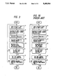
FIG. 14 shows an example of the neural network of a three-layer structure, wherein the input layer consists of P neurons 100(p) (p=1˜P), the hidden layer consists of Q neurons 200(q) (q=1˜Q) and the output layer consists of R neurons 300(r) (r=1˜R). In this example, P=4, Q=6 and R=2. The numbers of neurons included in the input and output layers depend on the number of input and output data, and the number of neurons of the hidden layer can arbitrarily be set.
FIG. 15 is a conceptual diagram showing a neuron (unit) which is an element of a neural network. Each neuron fetches data obtained by respectively multiplying a plurality of supplied data X(1)˜X(n) by each of weights W(1)˜W(n) as input data, and calculates a value "x" by subtracting a threshold value θ from the total sum ΣW(n)X(n) of them. And, as a transfer function f(x) with this "x" as a variable, a function which can be differentiated by "x" is used. A sigmoid function, a typical example of transfer function, is described in equation (1) in FIG. 24A.
The relationships between "x" and f(x) when coefficient "k" of the sigmoid function (hereinafter referred to as gradient "k") is assumed to be 0.1, 1.0 and 10 are shown in FIG. 16, and the differentiated value of the sigmoid function is shown in equation (2) in FIG. 24A.
With reference to FIG. 17, a learning algorithm by the conventional back propagation is now described. XO1(1), XO1(2), . . . XO1(P) are output data of the individual neurons 100(p) in the input layer, XO2(1), XO2(2), . . . XO2(Q) are output data of the individual neurons 200(q) in the hidden layer, XO3(1), XO3(2), . . . XO3(R) are output data of the individual neurons 300(r) in the output layer, XI2(1), XI2(3), . . . XI2(Q) are input data of the individual neurons 200(q) in the hidden layer, XI3(1), XI3(2), . . . XI3(R) are input data of the individual neurons 300(r) in the output layer, and T(1), T(2), . . . T(R) are training data.
W12 is weighting data for obtaining input data of the hidden layer from output data of the input layer, and W12(1,1) is weighting data when the output XO(1) is given to XI2(1,1) and WI2(2,2) is weighting data when the output XO1(2) is given to XI2(2) In general, W12(P,Q) is weighting data when XO1(P) is given to XI2(Q). Accordingly, although not shown, for instance, the weighting data when XO1(2) is given to XI2(1) is W12(2,1), and that when XO1(P) is given to XI2(1) is W12(p,1).
Similarly, W23 is weighting data for obtaining input data of the output layer from output data of the hidden layer, and in general, W23(Q,R) is weighting data when XO2(Q) is given to XI3(R). θ2(1), θ2(2), . . . θ2(Q) are threshold values of the hidden layer, and θ3(1), θ3(2), . . . θ3(R) are threshold values of the output layer.
XI2(1), input data of the hidden layer, is expressed by equation (3).
XI2(1)=XO1(1)×W12(1,1)+XO1(2)×W12(2,1) +. . . +XO1(P)×W12(P,1)                                    (3)
Similarly, XI2(Q) is expressed by equation (4).
XI2(Q)=XO1(1)×W12(1,Q)+XO1(2)×W12(2,Q) +. . . +XO1(P)×W12(P,Q)                                    (4)
XI3(1), input data of the output layer, is expressed by equation (5).
XI3(1)=XO2(1)×W23(1,1)+XO2(2)×W23(2,1) +. . . +XO2(Q)×W23(Q,1)                                    (5)
Similarly, XI3(R) is expressed by equation (6).
XI3(R)=XO2(1)×W23(1,R)+XO2(2)×W23(2,R) +. . . +XO2(Q)×W23(Q,R)                                    (6)
In the hidden layer, output data XO2(1) is obtained from input data XI2(1) by the equation (7). ##EQU1##
Similarly, the calculation for obtaining XO2(Q) from XI2(Q) is based on equation (8).
XO2(Q)=f{XI2(Q)-θ2(Q)}                               (8)
The calculation for obtaining XO3(1) from input data XI3(1)and the calculation for obtaining XO3(R) from input data XI3(R) are based on equations (9) and (10), respectively.
XO3(1)=f{XI3(1)-θ3(1)}                               (9)
XO3(R)=f{XI3(R)-θ3(R)}                               (10)
When output data XO3(r) (r=1˜R) have been obtained from the R neurons constituting the output layer for data XO1(p) (p=1˜P) given to the P neurons constituting the input layer, as described above, error data E are calculated on the basis of a predetermined cost function using the output data XO3(r) (r=1˜R) and training data T(r) (r=1˜R). When training data are used as in this example, such an error function as shown in equation (11) of FIG. 24A can be used as a cost function. Then, equations (12) to (15) are calculated using the error or cost function E.
Equations (12) to (15) of FIG. 24A represent partial differentiations of the error or cost function E by weighting variables W23(q,r), threshold variables θ3(r), weighting variables W12(p,q) and threshold variables θ2(q), respectively. That is, in equation (12), E is partially differentiated by all the combinations of W23(q,r) (all the combinations of q=1˜Q and r=1˜R, namely, W23(1,1), W23(2,1), . . . , W23(Q,1), W23(1,2), W23(2,2), . . . , W23(Q,2), . . . , W23(1,R), W23(2,R), . . . , W23(Q,R)). Similarly for equations (13) to (15), E is partially differentiated using all of the threshold variables θ3(r), weighting variables W12(p,q) and threshold variables θ2(q).
Then, the changing amount of current processing of each weighting data or threshold value ΔW12(p,q)0, Δθ2(q)0, ΔW23(q,r)0 and Δθ3(r)0 are determined from equations (16) to (19).
The various changing amounts in one time before (previous), two times before, . . . , and N times before precessings are discriminated by replacing the suffix 0 for the changing amount in current processing shown in equations (16) to (19) with 1˜N, as shown in equation (20). Further, the various changing coefficients in current, one time before, two times before, . . . , and N times before processings are determined by an equation (21).
These changing coefficients α0˜αN and β0˜βN may be preset to any values. The accumulated changing amounts ΔW12(p,q), Δθ2(q), ΔW23(q,r) and Δθ3(r) used in current processing are calculated from equations (22) to (25).
The accumulated changing amounts ΔW12(p,q), Δθ2(q), ΔW23(q,r) and Δθ3(r) calculated in this way are added to the weighting data and threshold value data W12(p,q), θ2(q), W23(q,r) and θ3(r), respectively, to correct them.
If there are "A" sets of combinations of input data and training data, those processings are repeated "A" times on all sets of said combinations. With this, one-time learning operation is finished. Predetermined times of such learnings are subsequently executed.
For example, for the learning of a problem of exclusive-OR (XOR) as shown in Table 1 described at the end of the specification, the numbers of neurons are two for the input layer and one for the output layer, and the hidden layer may have any number of neurons. In this example, the sets of the combinations of input data and training data is four.
As mentioned above, in the conventional back propagation operation, only weighting data and threshold values were subject to change by learning. The above described learning process is further described with reference to FIG. 18.
FIG. 18 is a flowchart showing an example of the learning algorithm according to the traditional back propagation operation.
In step S1, an input data pattern is selected (in the example of Table 1, one of four sets of input data is selected), and the selected data is supplied to the input layer.
In step S2, predetermined calculations are performed in the input hidden and output layers using the input data. By this, data (calculation result) is output from the output layer.
In step S3, the output data is compared with the training data corresponding to the selected input data, and error data "E" is calculated by equation (11).
In step S4, accumulated changing amounts ΔW12(p,q), Δθ2(q), ΔW23(q,r) and Δθ3(r) are calculated by equations (22) to (25).
In step S5, the calculated accumulated changing amounts are added to W12(p,q), θ2(q), W23(q,r) and θ3(r), which are weighting data and threshold value data, respectively, thereby to correct them.
In step S6, it is determined whether or not all of the input patterns have been selected. If all of the input patterns have not yet been selected, the process returns to step S1, and the process moves to step S7 if they have all been selected.
In step S7, it is determined that one learning operation has been completed.
In step S8, it is determined whether or not the learning has been completed predetermined times, and the process returns to step S1 if it has not been completed and terminates if it has been completed. Alternatively, in step S8, it may by determined whether or not output data can be obtained with precision higher than a pre-determined value, that is, whether or not the error data "E" has become smaller than a predetermined one.
The functions of the above described neural network is described more specifically using FIG. 19 in which input data and training data as shown in Table 1 are stored in an input/training data memory means 11, for instance. A selection means 12 sequentially transfers input data from the memory means 11 to neurons 100(p) of the input layer, and simultaneously sequentially outputs training data corresponding to the transferred input data to error calculation means 13.
Weighting calculation means 51 multiplies each output signal XO1(p) of neurons 100(p) by weighting data W12(p,q) stored in weighting data memory means 21 and outputs the result to each neuron 200(q) of the hidden layer. Similarly, weighting calculation means 52 multiplies each output signal XO2(q) of neurons 200(q) by weighting data W23(q,r) stored in weighting data memory means 22 and outputs the result to each neuron 300(r) of the output layer.
Transfer function calculation means 61 performs the calculations shown in equations (7), (8), etc. in each neuron 200(q), using the input data and the threshold values θ2(q) stored in threshold value memory means 31. Similarly, transfer function calculation means 62 performs the calculations shown in equations (9), (10), etc. within each neuron 300(r), using the input data and the threshold values θ3(r) stored in threshold value memory means 32.
The error calculation means 13 calculates error data "E" by performing the calculation of equation (11) using the training data and the data output from the output layer.
Accumulated changing amount calculation means 20 uses error data "E" and weighting data W12(p,q) to calculate accumulated changing amount ΔW12(p,q). In addition, using the error data "E" and weighting data W23(q,r), it calculates accumulated changing amount ΔW23(q,r).
Accumulated changing amount calculation means 30 uses error data "E" and threshold values θ2(q) to calculate accumulated changing amount Δθ2(q). Also, using the error data "E" and threshold values θ3(r), it calculates accumulated changing amount Δθ3(r).
The accumulated changing amounts ΔW12(p,q), Δθ2(q), ΔW23(q,r) and Δθ3(r) calculated in the individual accumulated changing amount calculation means 20 and 30 are added, in the adding means 23, 33, 24 and 34, respectively, to W12(p,q), θ2(q), W23(q,r) and θ3(r) which are the weighting data and threshold values respectively stored in the memory means 21, 31, 22 and 32. The weighting data and threshold values after the additions or change are stored again in the memory means 21, 31, 22 and 32.
In such conventional back propagation, the learning speed and precision of a neural network largely varied depending on the characteristics (in the case of a sigmoid function, the value of gradient "k") of the transfer function of individual neurons (in the above described example, sigmoid function), and sometimes the learning did not advance or the error could not converge.
A table 2 shows the result obtained by the learning of the problem of exclusive-OR as shown in Table 1 by a neural network which uses a sigmoid function as a transfer function according to the prior art. The neural network used in the learning comprises two neurons for the input layer, three neurons for the hidden layer and one neuron for the output layer. Table 2 shows the error sum of squares after the learning was performed ten thousand times respectively for the gradients "k" of the sigmoid function being fixed at 0.1, 1.0, 2.0, 3.0 and 10.0. The error sum of squares is the error data for one-time learning, namely, the mean value of four kinds of E's calculated when all of the four input patterns are supplied, and it is defined by equation (11).
As mentioned above, the learning speed and precision of the neural network greatly changes when the gradient "k" of the sigmoid function varies. Accordingly, a learning with high precision can be performed in a short time if the gradient "k" is set to an optimum value.
However, only the fact that the optimum value of the gradient "k" depends on the problem and the number of the neurons constituting the neural network has been revealed by the studies which have been made up to now, and the rule of trial and error must be applied for each problem to find the optimum value of "k", which is cumbersome and time-consuming. In addition, sufficient precision cannot be obtained unless the value of "k" is set at a different value for each neuron.
SUMMARY OF THE INVENTION
It is the object of the present invention to provide a neural network wherein the characteristics of the transfer function (gradient "k" for a sigmoid function, and various coefficients for other power or trigonometric function) can automatically be optimized independent of the problem to be solved and the number of the neurons constituting the network.
In the present invention, weighting data and threshold values are changed through learning, and at least one characteristic data (such as a coefficient) for determining the characteristics of the transfer function of each neuron is also changed through learning.
By changing each characteristic data through learning, the characteristics of each transfer function is optimized so as to be different for each neuron.
BRIEF DESCRIPTION OF THE DRAWING
FIG. 1 is a functional block diagram of an embodiment of the present invention.
FIG. 2 is a conceptual diagram for explaining a part of the learning algorithm of the embodiment of the present invention.
FIG. 3 is a flowchart showing the learning algorithm of the embodiment of the present invention.
FIG. 4 is a graph showing the convergence process when the problem of XOR was learned using the embodiment of the present invention.
FIG. 5 is a graph showing the convergence process when the problem of XOR was learned using conventional approach.
FIG. 6 is a graph showing the convergence process when the problem of XOR was learned according to another embodiment of the present invention.
FIG. 7 is a graph showing the convergence process when the problem of multiplication was learned using the embodiment of the present invention.
FIG. 8 is a graph showing the process when the problem of multiplication was learned using the conventional approach.
FIG. 9 is a graph showing an example of a special problem.
FIG. 10 is a graph showing the result when the example special problem of FIG. 9 was learned using the embodiment of the present invention.
FIG. 11 is a graph showing the convergence process when the example special problem of FIG. 9 was learned using the one embodiment of the present invention.
FIG. 12 is a graph showing the result when the example special problem of FIG. 9 was learned using the conventional approach.
FIG. 13 is a graph showing the process when the example special problem of FIG. 9 was learned using the conventional approach.
FIG. 14 is a diagram showing an example of the neural network of a three-layer structure.
FIG. 15 is a conceptual diagram showing a neuron which is an element of the neural network.
FIG. 16 is a representation showing an example characteristic of a sigmoid function.
FIG. 17 is a conceptual diagram for explaining the main part of the learning algorithm according to the conventional back propagation.
FIG. 18 is a flowchart showing an example of the learning algorithm according to the conventional back propagation.
FIG. 19 is a functional block diagram of the conventional neural network.
FIG. 20 is a graph showing the positions of the input points of a periodic function to be interpolated and the interpolated periodic function waveform.
FIG. 21 is a graph showing the convergence process when the periodic function problem was learned using still another embodiment of the present invention.
FIG. 22 is a graph showing the convergence process when the same periodic function problem as FIG. 21 was learned using the conventional approach.
FIG. 23 is a periodic function waveform of the learning result by the approach shown in FIG. 22.
FIGS. 24A-24D describe equations 1, 2, 11-34 which are used for the present invention.
DETAILED DESCRIPTION OF THE PREFERRED EMBODIMENT
The present invention is now described in detail with reference to the drawings.
FIG. 2 is a conceptual diagram for explaining the main part of the learning algorithm according to one embodiment of the present invention. In the figure, the same symbols as in FIG. 17 represent the same or equivalent portions.
The transfer function of the individual neurons constituting the hidden layer is a sigmoid function expressed by equation (1), and k2(q) (q=1˜Q) represents the gradient of the sigmoid function similarly to "k" in the equation (1). The variable "x" of the sigmoid function of the hidden layer is {XI2(q)-θ2(q)} (q=1˜Q).
Similarly, the transfer function of the individual neurons constituting the output layer is also a sigmoid function, and k3(r) (r=1˜R) represents the gradient thereof. The variable "x" of the sigmoid function of the output layer is {X13(r)˜θ3(r)} (r=1˜R).
In a neural network having the above-mentioned construction, error data "E" is calculated from equation (11). Using the error or cost function "E", equations (12) to (15) are calculated. Of course, in this case, the calculations are performed for all the combinations of each of variables W23(q,r), θ3(r), W12(p,q) and θ2(q) (p=1˜P, q=1˜Q, r=1˜R) as described above. Equations (26) and (27) are also calculated. These calculations are also performed for all the combinations of each of variables k3(r) and k2(q) (r=1˜R, q=1˜Q).
Then, the changing amounts of current processing of the respective weighting data and threshold values ΔW12(p,q)0, Δθ2(q)0, ΔW23(q,r)0 and Δθ3(r)0 are determined by equations (16) to (19).
Similarly, the changing amounts of current processing Δk2(q)0 and Δk3(r)0 for the respective gradients k2 and k3 are determined by equations (28) and (29). In addition, the various changing amounts in the one-time-before (previous), two-time-before, . . . , N-time-before processings are discriminated by replacing the suffix 0 of the changing amount of current processing by 1˜N, as shown in equations (20) to (30).
The various changing coefficients in the current, one-time-before, two-time-before, . . . , N-time-before processings are determined as shown in equations (21) and (31). Each of the changing coefficients α0˜αN, β0˜βN and γ0˜γN may be preset to any value. The accumulated changing amounts ΔW12(p,q), Δθ2(q), ΔW23(q,r) and Δθ3(r) used in current processing are calculated by equations (22) to (25), and the accumulated changing amounts Δk2(q) and Δk3(r) are calculated from equations (32) and (33).
The accumulated changing amounts ΔW12(p,q), Δθ2(q), ΔW23(q,r), Δθ3(r), Δk2(q) and Δk3(r) calculated in the described method are respectively added to the weighting data and threshold values W12(p,q), θ2(q), W23(q,r) and θ3(r), and gradients k2(q) and k3(r) to correct them. In equations (22) to (25) and equations (32) and (33), each accumulated changing amount may be calculated using the changing amount of current processing and that of at least one time before processing.
If there are "A" sets of combinations of the input data and training data, these processings are performed A-times for all the combinations. With this, one-time learning is completed. Such learning is subsequently executed predetermined times.
The learning algorithm in the embodiment of the present invention changes or corrects the weighting data, threshold values and gradients at step S5A, as shown in the flowchart of FIG. 3. Of course, in the previous step S4A, the accumulated changing amounts Δk2(q) and Δk3(r) for changing gradients are also calculated in addition to the accumulated amounts calculated in the prior art.
If "x" and "k" of the sigmoid function expressed by equation (1) are variables, partial differentiations by "x" and "k" can be expressed by equation (34).
The embodiment of the present invention is described more specifically with reference to the functional block diagram of FIG. 1 in which the same symbols as in FIG. 19 represent the same or equivalent portions.
In FIG. 1, the transfer function calculation means 61 and 62 perform calculations using sigmoid functions as described in connection with FIG. 19. The gradients k2(q) and k3(r) of the sigmoid functions are stored in the gradient memory means 41 and 42, respectively.
Accumulated changing amount calculation mean 40 calculates accumulated changing amount Δk2(q) using the error data "E" and gradient k2(q). In addition, using the "E" and gradient k3(r), the accumulated changing amount Δk3(r) is calculated. The accumulated changing amounts Δk2(q) and Δk3(r) are added to the gradients k2(q) and k3(r) stored in memory means 41 and 42 in adding means 43 and 44. The gradients corrected by the addition are newly stored in the memory means 41 and 42 for gradient correction.
The present inventors calculated various problems using the neural network according to the learning algorithm as described above. Several calculation results are shown below.
(1) XOR
FIG. 4 shows a convergence state, which was obtained when the problem of XOR shown in Table 1 was learned by the approach of the present invention, using a neural network consisting of a two-neuron input layer, three-neuron hidden layer and one-neuron output layer. The transfer function of each neuron is a sigmoid function, and in FIG. 4, the relationship between the number of times of learning (abscissa) and error sum of squares (ordinate) is shown. For the purpose of comparison the relationship between the number of times of learning (abscissa) and error sum of squares ordinate) according to the conventional method, in which the gradient "k" of the sigmoid function is not learned, is shown in FIG. 5. FIG. 5 is an example for k=2.
In Table 3, learning precision obtained by ten thousand times learnings, that is the error sum of squares, and calculation time required for that are shown. For calculation, a workstation of 20 [MIPS] was used.
Table 4 shows the number of times of learning required before the error sum of squares 1×10⁻⁴ was obtained and the calculation time spent for that. As seen from these tables, regarding the problem of XOR, the learning precision could be increased by 10 to 100 times for the same number of times of learning as compared with the conventional method in accordance with the embodiment of the present invention, and the number of times of learning for obtaining the same learning precision can be decreased by at least 1/3 to 1/4 times (1/2 to 1/3 times in calculation time) as compared with the conventional method.
(2) Multiplication
FIG. 7 shows a learning process when a problem of multiplication as shown in Table 7 was learned by the technique of the present invention using a neural network, which consists of a two-neuron input layer, a nine-neuron hidden layer and a single-neuron output layer. The transfer function of each neuron is a sigmoid function. In FIG. 7, the relationship between the number of times of learning (abscissa) and error sum of squares (ordinate) is shown as in FIGS. 4 and 5.
The relationship between the number of times of learning (abscissa) and error sum of squares (ordinate) according to the conventional approach is shown for comparison in FIG. 8. FIG. 8 is an example for k=2.
As seen from the comparison of the two figures, even a problem for which learning precision was hardly increased by the conventional approach can be learned up to considerable precision in the present invention.
(3) Special problem
The result of a learning of a functional relation as shown in FIG. 9 is described below. The network used consists of one neuron for the input layer, seven neurons for the hidden layer and one neuron for the output layer, and the transfer function of each neuron is a sigmoid function.
Table 5 shows the calculation result of the embodiment of the present invention, in which error sums of squares are shown with a changing coefficient of α=0.9 and the changing coefficients β and γ being parameters.
In table 5, each of marks `×` indicates that convergence was not achieved because of a too large error and learning could not be made at last, each of marks `Δ` indicates that the converged error sum of squares was in the order of 0.1×10⁻⁵, each of marks `◯` indicates that the converged error sum of squares was in the order of 0.1×10⁻⁶, and a mark `⊚` indicates that the converged error sum of squares was the smallest and its value was 0.278×10⁻⁶. The input and output data for the best case are shown in FIG. 10. In FIG. 11, the relationship between the number of times of learning (abscissa) and error sum of squares (ordinate) is shown, as in FIGS. 4 and 5.
For the purpose of comparison, the calculation result by the conventional approach is shown in Table 6. Table 6 shows error sums of squares when the changing coefficients α and β are parameters. The relation between the input and output data for α=0.1 and β=0.1 which provided the smallest error sum of squares is shown in FIG. 12. In FIG. 13, the relationship between the number of times of learning (abscissa) and error sum of squares (ordinate) is shown.
It will be realized from the foregoing that the problem of FIG. 9 can be learned by the present invention with considerable high precision, though it can be hardly learned by the conventional learning technique.
Now, description is made of another embodiment in which a power function is used as the transfer function.
(4) XOR of Table 1
The neural network used consists of two neurons for the input layer, two neurons for the hidden layer and one neuron for the output layer, and the transfer function of each neuron is a power function (axb +c). Two coefficients b1 and b2 of the power functions for the two neurons of the hidden layer were set at 1.0 and 2.0, respectively, and constants a1 and a2, and c1 and c2 were learned. FIG. 6 shows the attenuation state of the error sum of squares (ordinate) vs. the number of times of learning (abscissa). Table 8 shows the result of a thousand times learnings. The error sum of squares for this was 1.40×10⁻¹³, and the required calculation time was 0.93 sec. For the purpose of comparison, the result of a thousand times learnings performed in the conventional method using a sigmoid function is shown in Table 9. The error sum of squares for said result was 7.31×10⁻⁵, and the required calculation time was 1.15 sec. It is understood from these comparisons that a learning with higher precision can be accomplished by the present invention in a shorter time.
(5) Interpolation of periodic function
Description is made of a further embodiment of the present invention in which a trigonometric function is used as the transfer function. The exercise is to obtain a periodic function which interpolates a periodic function, in which output values (ordinate) are given corresponding to discrete values of input (abscissa) as shown in Table 10 and by black points in FIG. 20. The network used consists of one neuron for the input layer, two neurons for the hidden layer and one neuron for the output layer, the transfer function of each neuron is a trigonometric function {a Sin(cx)+b Sin(dx)}, and all constants in the trigonometric function were learned.
The relationship between the number of times of learning (abscissa) and error sum of squares (ordinate) is shown in FIG. 21. The error sum of squares after ten thousand times learnings was 6.07×10⁻⁷, and the required time was 88 sec. The waveform of the periodic function obtained by the learning is shown by a dotted line in FIG. 20. For comparison, the result of a hundred thousand times learnings by the conventional method using a sigmoid function, which is similar to FIG. 21, is shown in FIG. 22. The error sum of squares after the hundred thousand times learnings was 1.13×10⁻², and the required time was 21 sec. It is seen from FIG. 22 that the error sum of squares does not readily decrease. Also, the waveform of the periodic function obtained by the prior art learning, which corresponds to FIG. 20, is shown in FIG. 23. As seen from the comparison of FIGS. 20 and 23, and/or FIGS. 21 and 22, a learning with higher precision can be performed by the present invention in a shorter time.
Although, in the above description, the learning (changing) of the weighting data, threshold values and gradients are performed by adding accumulated changing amounts of past changing amounts to the weighting data, threshold values and gradients, as shown in equations (22) to (25) and equations (32) and (33), the learning may be made using only the changing amounts of current processing.
Moreover, in the above described embodiments, the changing coefficients α, β and γ are common for the weighting data, threshold values and gradients of each of the hidden and output layers, but coefficients different among layers and/or neurons may be used.
In the above described embodiments, if there are a plurality of input data and training data as shown in Table 1 and FIG. 6, the combination of input data and training data are sequentially selected out of them and are calculated as shown in FIG. 3, and it is determined that one learning has been completed when the calculations have been performed using all the sets of input data and training data. As a result, all combinations of input and training data are evenly used to perform the learning. However, for instance, data may be selected at random from a plurality of input and training data to perform a learning, without evenly using data.
Although the weighting data, threshold values and gradients were to be corrected each time error data is detected in the foregoing description, the changing amounts (or the accumulated changing amounts) used for correction may be stored, and when the learning has been completed a predetermined number of times, they may be collectively added to the weighting data, threshold values and gradients to make data correction.
Although the foregoing description has been made to the effect that error data "E" is calculated using training data with an error function as shown in equation (11) being as a cost function, it is also possible that an appropriate cost function is used instead of training data and the learning is made so that the calculation result of the cost function becomes a predetermined value (for instance, the smallest value).
The above described various calculations can be executed by software using a microcomputer, but they may be accomplished instead by hardware circuit networks.
As apparent from the above description, in accordance with the present invention, at least one characteristic data which determines the characteristics of the transfer function of each neuron is to be learned, and thus the transfer function characteristics are different for each neuron independently of the nature of a problem and/or the number of neurons and become optimum. Accordingly, a learning with high precision can be performed in a short time.
If it is taken into consideration that neural networks have been studied on the analogy of the neural circuit networks of living things and the individual nerve cells of a living thing are not always uniform in the same and single living body, it can be said that the learning system of the present invention is quite appropriate.
              TABLE 1                                                     
______________________________________                                    
                  Training                                                
Input             Data                                                    
X (1)          X (2)  Y                                                   
______________________________________                                    
0              1      1                                                   
1              0      1                                                   
0              0      0                                                   
1              1      0                                                   
______________________________________                                    
              TABLE 2                                                     
______________________________________                                    
Gradient of    Error Sum of Squares                                       
Sigmoid Function                                                          
               After 10000 Learnings                                      
______________________________________                                    
0.1            2.5 × 10.sup.-1                                      
1.0            1.6 × 10.sup.-4                                      
2.0            3.3 × 10.sup.-5                                      
3.0            2.3 × 10.sup.-5                                      
10.0           5.0 × 10.sup.-1                                      
______________________________________                                    
              TABLE 3                                                     
______________________________________                                    
                          Calculation                                     
            Error Sum of Squares                                          
                          Time [sec]                                      
______________________________________                                    
Conventional Method                                                       
              0.326 × 10.sup.-4                                     
                              5.45                                        
Present Invention                                                         
              0.506 × 10.sup.-5                                     
                              5.84                                        
______________________________________                                    
              TABLE 4                                                     
______________________________________                                    
             Number of Times of                                           
                           Calculation                                    
             Learning      Time [sec]                                     
______________________________________                                    
Conventional Method                                                       
               3592            1.99                                       
Present Invention                                                         
               1184            0.73                                       
______________________________________                                    
              TABLE 5                                                     
______________________________________                                    
α  = 0.9                                                            
Changing  Changing Coefficient γ                                    
Coefficient                                                               
          0.1        0.3   0.5     0.7 0.9                                
______________________________________                                    
β                                                                    
0.1       Δ    Δ                                              
                           x       x   x                                  
0.3       Δ    x     x       x   x                                  
0.5       x          x     ∘                                  
                                   ⊚                       
                                       ∘                      
0.7       x          x     ∘                                  
                                   ∘                          
                                       ∘                      
0.9       x          x     x       Δ                                
                                       Δ                            
______________________________________                                    
              TABLE 6                                                     
______________________________________                                    
Changing  Changing Coefficient β                                     
Coefficient                                                               
          0.1      0.3    0.5     0.7  0.9                                
______________________________________                                    
α                                                                   
0.1       0.147    0.159  0.171   0.172                                   
                                       0.173                              
0.3       0.159    0.161  0.167   0.173                                   
                                       0.178                              
0.5       0.171    0.172  0.173   0.174                                   
                                       0.177                              
0.7       0.175    0.176  0.176   0.177                                   
                                       0.177                              
0.9       0.178    0.178  0.179   0.179                                   
                                       0.179                              
______________________________________                                    
              TABLE 7                                                     
______________________________________                                    
Input             Training                                                
X (1)          X (2)  Data Y                                              
______________________________________                                    
0              0      0                                                   
1              0      0                                                   
2              0      0                                                   
3              0      0                                                   
4              0      0                                                   
5              0      0                                                   
0              1      0                                                   
1              1      1                                                   
2              1      2                                                   
3              1      3                                                   
4              1      4                                                   
5              1      5                                                   
0              2      0                                                   
1              2      2                                                   
2              2      4                                                   
3              2      6                                                   
4              2      8                                                   
5              2      10                                                  
0              3      0                                                   
1              3      3                                                   
2              3      6                                                   
3              3      9                                                   
4              3      12                                                  
5              3      15                                                  
0              4      0                                                   
1              4      4                                                   
2              4      8                                                   
3              4      12                                                  
4              4      16                                                  
5              4      20                                                  
0              5      0                                                   
1              5      5                                                   
2              5      10                                                  
3              5      15                                                  
4              5      20                                                  
5              5      25                                                  
______________________________________                                    
              TABLE 8                                                     
______________________________________                                    
Input               Output                                                
X (1)           X (2)   Y                                                 
______________________________________                                    
0.00000         0.00000 0.00000                                           
0.00000         1.00000 1.00000                                           
1.00000         0.00000 1.00000                                           
1.00000         1.00000 0.00000                                           
______________________________________                                    
              TABLE 9                                                     
______________________________________                                    
Input               Output                                                
X (1)           X (2)   Y                                                 
______________________________________                                    
0.00000         0.00000 0.00985                                           
0.00000         1.00000 0.97118                                           
1.00000         0.00000 0.97214                                           
1.00000         1.00000 0.03446                                           
______________________________________                                    
              TABLE 10                                                    
______________________________________                                    
                Training                                                  
Input           Data                                                      
______________________________________                                    
 -10.000 -9.372 -8.743 -8.115 -7.487 -6.858 -6.230 -5.602 -4.973 -4.345   
-3.717 -3.088 -2.460 -1.832 -1.204 -0.575 +0.053 +0.681 +1.310 +1.938     
                 -1.542 +0.185  +1.623 +0.388 -2.165 -2.785 -0.788 +1.014 
                +0.204 -1.907 -2.110 +0.239 +2.291 +1.607 -0.516 -0.867   
                +1.212 +2.899 +1.791 -0.774                               
                           ##STR1##                                       
+2.566          -1.542                                                    
+3.195          +0.185                                                    
+3.823          +1.623                                                    
+4.451          +0.388                                                    
+5.080          -2.165                                                    
+5.708          -2.785                                                    
+6.336          -0.788                                                    
+6.965          +1.014                                                    
+7.593          +0.204                                                    
+8.221          -1.907                                                    
+8.850          -2.110                                                    
+9.478          +0.239                                                    
______________________________________                                    

Claims (11)

What is claimed is:
1. A neural network comprising a plurality of neurons each performing a signal processing corresponding to a neural element, said neurons being hierarchically connected in the order of at least one input layer, at least one hidden layer and an output layer, and said input layer, hidden layer and output layer each consisting of at least one neuron, individual neurons of said hidden layer and output layer being operative to correct the data weighted by multiplying the outputs of the preceding input layer or hidden layer by predetermined weighting data with a predetermined threshold value, respectively, and to substitute the data after the correction in a predetermined transfer function to calculate output data, said neural network including:
error data calculation means operative to use a predetermined cost function to calculate error data from the output data of the output layer,
weighting data correction means operative to partially differentiate said cost function with each of a plurality of weighting variables to obtain partial differentiated coefficients, and to correct said weighting data according to said partial differential coefficients.
threshold value correction means operative to partially differentiate said cost function with each of a plurality of threshold variables to obtain partial differentiated coefficients, and to correct each said threshold value according to said partial differential coefficients, and
characteristic data correction means for partially differentiating said cost function, to obtain partial differentiated coefficients, with at least one characteristic variable that determines the characteristics of the respective transfer functions of said hidden layer and said output layer, and operative to correct said characteristic data according to said partial differential coefficients.
2. A neural network as set forth in claim 1 wherein said characteristic data correction means corrects said characteristic data using the partial differential coefficients obtained by partially differentiating said cost function with said at least one characteristic variable, and the previous values of said partial differential coefficients.
3. A neural network as set forth in claim 2 wherein said cost function is an error function, and said error data calculation means compares the data output from said output layer with training data corresponding to the input data supplied to said input layer and applies the comparison result to said error function, thereby to calculate error data.
4. A neural network as set forth in claim 2 wherein said weighting data correction means uses the partially differentiated value of said cost function by said weighting variables and the previous value of said partially differentiated value to correct said weighting data.
5. A neural network as set forth in claim 2 wherein said threshold value correction means uses the partially differentiated variables of said cost function by said threshold value and the previous value of said partially differentiated value to correct said threshold value.
6. A neural network as set forth in claim 1 wherein said transfer function is a sigmoid function and said characteristic variable is the gradient of the sigmoid function.
7. A neural network as set forth in claim 1 wherein said transfer function is a power function (axb +c) and said characteristic variable is at least one constant of said power function.
8. A neural network as set forth in claim 1 wherein said transfer function is a trigonometric function {a Sin(cx)+b Cos(dx)} and said characteristic variable is at least one constant of said trigonometric function.
9. A neural network as set forth in claim 1 wherein said cost function is an error function, and said error data calculation means compares the data output from said output layer with training data corresponding to the input data supplied to said input layer and applies the comparison result to said error function, thereby to calculate error data.
10. A neural network as set forth in claim 1 wherein said weighting data correction means uses the partially differentiated value of said cost function by said weighting variables and the previous value of said partially differentiated value to correct said weighting data.
11. A neural network as set forth in claim 1 wherein said threshold value correction means uses the partially differentiated value of said cost function by said threshold variables and the previous value of said partially differentiated value to correct said threshold value.
US07/836,593 1991-02-20 1992-02-18 Neural network having an optimized transfer function for each neuron Expired - Fee Related US5280564A (en)

Applications Claiming Priority (2)

Application Number Priority Date Filing Date Title
JP3-45613 1991-02-20
JP3045613A JPH04266153A (en) 1991-02-20 1991-02-20 Neural network

Publications (1)

Publication Number Publication Date
US5280564A true US5280564A (en) 1994-01-18

Family

ID=12724227

Family Applications (1)

Application Number Title Priority Date Filing Date
US07/836,593 Expired - Fee Related US5280564A (en) 1991-02-20 1992-02-18 Neural network having an optimized transfer function for each neuron

Country Status (2)

Country Link
US (1) US5280564A (en)
JP (1) JPH04266153A (en)

Cited By (19)

* Cited by examiner, † Cited by third party
Publication number Priority date Publication date Assignee Title
US5452402A (en) * 1992-11-26 1995-09-19 Matsushita Electric Industrial Co., Ltd. Neural network circuit for adaptively controlling the coupling of neurons
US5486999A (en) * 1994-04-20 1996-01-23 Mebane; Andrew H. Apparatus and method for categorizing health care utilization
US5630019A (en) * 1992-05-23 1997-05-13 Kabushiki Kaisha Topcon Waveform evaluating apparatus using neural network
US5649067A (en) * 1992-12-16 1997-07-15 U.S. Philips Corporation Neural device and method of constructing the device
US5796923A (en) * 1991-12-27 1998-08-18 Daikin Industries, Ltd. Methods and apparatus for estimating unknown quantities
US5812992A (en) * 1995-05-24 1998-09-22 David Sarnoff Research Center Inc. Method and system for training a neural network with adaptive weight updating and adaptive pruning in principal component space
US6513023B1 (en) 1999-10-01 2003-01-28 The United States Of America As Represented By The Administrator Of The National Aeronautics And Space Administration Artificial neural network with hardware training and hardware refresh
EP1283496A2 (en) * 2001-08-11 2003-02-12 deneg GmbH Method for generating neural networks
US20040064426A1 (en) * 2002-09-30 2004-04-01 Depold Hans R. Physics based neural network for validating data
US20040064425A1 (en) * 2002-09-30 2004-04-01 Depold Hans R. Physics based neural network
US20040064427A1 (en) * 2002-09-30 2004-04-01 Depold Hans R. Physics based neural network for isolating faults
WO2014025765A2 (en) * 2012-08-06 2014-02-13 University Of Miami Systems and methods for adaptive neural decoding
WO2018076331A1 (en) * 2016-10-31 2018-05-03 北京中科寒武纪科技有限公司 Neural network training method and apparatus
US10915298B1 (en) 2019-10-08 2021-02-09 Ali Tasdighi Far Current mode multiply-accumulate for compute in memory binarized neural networks
US11144316B1 (en) 2018-04-17 2021-10-12 Ali Tasdighi Far Current-mode mixed-signal SRAM based compute-in-memory for low power machine learning
US11488007B2 (en) 2019-12-06 2022-11-01 International Business Machines Corporation Building of custom convolution filter for a neural network using an automated evolutionary process
US11593664B2 (en) * 2019-07-10 2023-02-28 Stmicroelectronics (Rousset) Sas Method and computational tool for determining transfer functions between pairs of successive layers of a neural network
US11610104B1 (en) 2019-12-30 2023-03-21 Ali Tasdighi Far Asynchronous analog accelerator for fully connected artificial neural networks
US11615256B1 (en) 2019-12-30 2023-03-28 Ali Tasdighi Far Hybrid accumulation method in multiply-accumulate for machine learning

Families Citing this family (1)

* Cited by examiner, † Cited by third party
Publication number Priority date Publication date Assignee Title
JP5513960B2 (en) * 2010-04-12 2014-06-04 株式会社メガチップス Image processing device

Citations (10)

* Cited by examiner, † Cited by third party
Publication number Priority date Publication date Assignee Title
US4945494A (en) * 1989-03-02 1990-07-31 Texas Instruments Incorporated Neural network and system
JPH0336659A (en) * 1989-07-04 1991-02-18 Omron Corp Learning controller for hierarchical neural network
JPH0390956A (en) * 1989-08-31 1991-04-16 Fujitsu Ltd Information processor
US5043913A (en) * 1988-06-14 1991-08-27 Mitsubishi Denki Kabushiki Kaisha Neural network
US5046020A (en) * 1988-12-16 1991-09-03 E. I. Du Pont De Nemours And Company Distributed parallel processing network wherein the connection weights are generated using stiff differential equations
US5113483A (en) * 1990-06-15 1992-05-12 Microelectronics And Computer Technology Corporation Neural network with semi-localized non-linear mapping of the input space
US5119469A (en) * 1989-05-17 1992-06-02 United States Of America Neural network with weight adjustment based on prior history of input signals
US5134685A (en) * 1990-02-06 1992-07-28 Westinghouse Electric Corp. Neural node, a netowrk and a chaotic annealing optimization method for the network
US5167006A (en) * 1989-12-29 1992-11-24 Ricoh Company, Ltd. Neuron unit, neural network and signal processing method
US5187680A (en) * 1989-06-15 1993-02-16 General Electric Company Neural net using capacitive structures connecting input lines and differentially sensed output line pairs

Patent Citations (10)

* Cited by examiner, † Cited by third party
Publication number Priority date Publication date Assignee Title
US5043913A (en) * 1988-06-14 1991-08-27 Mitsubishi Denki Kabushiki Kaisha Neural network
US5046020A (en) * 1988-12-16 1991-09-03 E. I. Du Pont De Nemours And Company Distributed parallel processing network wherein the connection weights are generated using stiff differential equations
US4945494A (en) * 1989-03-02 1990-07-31 Texas Instruments Incorporated Neural network and system
US5119469A (en) * 1989-05-17 1992-06-02 United States Of America Neural network with weight adjustment based on prior history of input signals
US5187680A (en) * 1989-06-15 1993-02-16 General Electric Company Neural net using capacitive structures connecting input lines and differentially sensed output line pairs
JPH0336659A (en) * 1989-07-04 1991-02-18 Omron Corp Learning controller for hierarchical neural network
JPH0390956A (en) * 1989-08-31 1991-04-16 Fujitsu Ltd Information processor
US5167006A (en) * 1989-12-29 1992-11-24 Ricoh Company, Ltd. Neuron unit, neural network and signal processing method
US5134685A (en) * 1990-02-06 1992-07-28 Westinghouse Electric Corp. Neural node, a netowrk and a chaotic annealing optimization method for the network
US5113483A (en) * 1990-06-15 1992-05-12 Microelectronics And Computer Technology Corporation Neural network with semi-localized non-linear mapping of the input space

Cited By (22)

* Cited by examiner, † Cited by third party
Publication number Priority date Publication date Assignee Title
US5796923A (en) * 1991-12-27 1998-08-18 Daikin Industries, Ltd. Methods and apparatus for estimating unknown quantities
US5630019A (en) * 1992-05-23 1997-05-13 Kabushiki Kaisha Topcon Waveform evaluating apparatus using neural network
US5452402A (en) * 1992-11-26 1995-09-19 Matsushita Electric Industrial Co., Ltd. Neural network circuit for adaptively controlling the coupling of neurons
US5649067A (en) * 1992-12-16 1997-07-15 U.S. Philips Corporation Neural device and method of constructing the device
US5802507A (en) * 1992-12-16 1998-09-01 U.S. Philips Corporation Method for constructing a neural device for classification of objects
US5486999A (en) * 1994-04-20 1996-01-23 Mebane; Andrew H. Apparatus and method for categorizing health care utilization
US5812992A (en) * 1995-05-24 1998-09-22 David Sarnoff Research Center Inc. Method and system for training a neural network with adaptive weight updating and adaptive pruning in principal component space
US6513023B1 (en) 1999-10-01 2003-01-28 The United States Of America As Represented By The Administrator Of The National Aeronautics And Space Administration Artificial neural network with hardware training and hardware refresh
EP1283496A2 (en) * 2001-08-11 2003-02-12 deneg GmbH Method for generating neural networks
EP1283496A3 (en) * 2001-08-11 2006-03-08 KISTERS Aktiengesellschaft Method for generating neural networks
US20040064425A1 (en) * 2002-09-30 2004-04-01 Depold Hans R. Physics based neural network
US20040064427A1 (en) * 2002-09-30 2004-04-01 Depold Hans R. Physics based neural network for isolating faults
US20040064426A1 (en) * 2002-09-30 2004-04-01 Depold Hans R. Physics based neural network for validating data
WO2014025765A2 (en) * 2012-08-06 2014-02-13 University Of Miami Systems and methods for adaptive neural decoding
WO2014025765A3 (en) * 2012-08-06 2014-05-01 University Of Miami Systems and methods for adaptive neural decoding
WO2018076331A1 (en) * 2016-10-31 2018-05-03 北京中科寒武纪科技有限公司 Neural network training method and apparatus
US11144316B1 (en) 2018-04-17 2021-10-12 Ali Tasdighi Far Current-mode mixed-signal SRAM based compute-in-memory for low power machine learning
US11593664B2 (en) * 2019-07-10 2023-02-28 Stmicroelectronics (Rousset) Sas Method and computational tool for determining transfer functions between pairs of successive layers of a neural network
US10915298B1 (en) 2019-10-08 2021-02-09 Ali Tasdighi Far Current mode multiply-accumulate for compute in memory binarized neural networks
US11488007B2 (en) 2019-12-06 2022-11-01 International Business Machines Corporation Building of custom convolution filter for a neural network using an automated evolutionary process
US11610104B1 (en) 2019-12-30 2023-03-21 Ali Tasdighi Far Asynchronous analog accelerator for fully connected artificial neural networks
US11615256B1 (en) 2019-12-30 2023-03-28 Ali Tasdighi Far Hybrid accumulation method in multiply-accumulate for machine learning

Also Published As

Publication number Publication date
JPH04266153A (en) 1992-09-22

Similar Documents

Publication Publication Date Title
US5280564A (en) Neural network having an optimized transfer function for each neuron
Ivakhnenko Polynomial theory of complex systems
Bontempi et al. The local paradigm for modeling and control: from neuro-fuzzy to lazy learning
Gorinevsky et al. Comparison of some neural network and scattered data approximations: The inverse manipulator kinematics example
Khan et al. Neufuz: Neural network based fuzzy logic design algorithms
US5630023A (en) Signal processor
US5222194A (en) Neural network with modification of neuron weights and reaction coefficient
Jovanovic et al. Modified ANFIS architecture-improving efficiency of ANFIS technique
EP0907117A1 (en) Nonlinear neural predictive control system
Kim A design of CMAC-based fuzzy logic controller with fast learning and accurate approximation
US5239618A (en) Data processing device with network structure and its learning processing method
Terziyska et al. Implicit GPC based on semi fuzzy neural network model
Cavalieri et al. Improving Hopfield neural network performance by fuzzy logic-based coefficient tuning
CN113485099A (en) Online learning control method of nonlinear discrete time system
Siddikov et al. Structural-parametric adaptation of fuzzy-logical control system
Fravolini et al. Comparison of different growing radial basis functions algorithms for control systems applications
JPH04291662A (en) Operation element constituted of hierarchical network
JP3733711B2 (en) Simplified quasi-Newton projection calculation system, neural network learning system, recording medium, and signal processing apparatus
Otadi Simulation and evaluation of second-order fuzzy boundary value problems
US5528729A (en) Neural network learning apparatus and learning method
JPH05128285A (en) Neuro-processor
Zhang et al. Adaptive RBF neural-networks control for discrete nonlinear systems based on data
Rezaee-Ahmadi et al. Z-adaptive fuzzy inference systems
Kim et al. Stable neural controller design based on composite adaptation
Deibel et al. Fuzzy logic learning algorithm for identifying inverse dynamics of a system

Legal Events

Date Code Title Description
AS Assignment

Owner name: HONDA GIKEN KOGYO KABUSHIKI KAISHA A COMPANY OF J

Free format text: ASSIGNMENT OF ASSIGNORS INTEREST.;ASSIGNORS:SHIOMI, KAZUYUKI;WATANABE, SEI;REEL/FRAME:006020/0584

Effective date: 19920127

REFU Refund

Free format text: REFUND - PAYMENT OF MAINTENANCE FEE, 4TH YR, SMALL ENTITY (ORIGINAL EVENT CODE: R283); ENTITY STATUS OF PATENT OWNER: LARGE ENTITY

FEPP Fee payment procedure

Free format text: PAT HLDR NO LONGER CLAIMS SMALL ENT STAT AS INDIV INVENTOR (ORIGINAL EVENT CODE: LSM1); ENTITY STATUS OF PATENT OWNER: LARGE ENTITY

FPAY Fee payment

Year of fee payment: 4

FPAY Fee payment

Year of fee payment: 8

REMI Maintenance fee reminder mailed
LAPS Lapse for failure to pay maintenance fees
STCH Information on status: patent discontinuation

Free format text: PATENT EXPIRED DUE TO NONPAYMENT OF MAINTENANCE FEES UNDER 37 CFR 1.362

FP Lapsed due to failure to pay maintenance fee

Effective date: 20060118