US7088457B1 - Iterative least-squares wavefront estimation for general pupil shapes - Google Patents
Iterative least-squares wavefront estimation for general pupil shapes Download PDFInfo
- Publication number
- US7088457B1 US7088457B1 US10/867,527 US86752704A US7088457B1 US 7088457 B1 US7088457 B1 US 7088457B1 US 86752704 A US86752704 A US 86752704A US 7088457 B1 US7088457 B1 US 7088457B1
- Authority
- US
- United States
- Prior art keywords
- wavefront
- slope
- pupil
- data
- iterations
- Prior art date
- Legal status (The legal status is an assumption and is not a legal conclusion. Google has not performed a legal analysis and makes no representation as to the accuracy of the status listed.)
- Active, expires
Links
- 210000001747 pupil Anatomy 0.000 title claims abstract description 80
- 238000000034 method Methods 0.000 claims abstract description 84
- 230000001788 irregular Effects 0.000 claims abstract description 8
- 239000011159 matrix material Substances 0.000 claims description 61
- 238000000605 extraction Methods 0.000 claims description 7
- 230000002950 deficient Effects 0.000 claims description 3
- 238000013213 extrapolation Methods 0.000 claims description 3
- 238000005070 sampling Methods 0.000 abstract description 16
- 230000003287 optical effect Effects 0.000 description 22
- 238000012360 testing method Methods 0.000 description 21
- 238000005259 measurement Methods 0.000 description 16
- 230000003044 adaptive effect Effects 0.000 description 11
- 238000000354 decomposition reaction Methods 0.000 description 9
- 238000004458 analytical method Methods 0.000 description 8
- 230000006870 function Effects 0.000 description 8
- 238000013459 approach Methods 0.000 description 7
- 238000012804 iterative process Methods 0.000 description 7
- 230000008901 benefit Effects 0.000 description 4
- 238000010276 construction Methods 0.000 description 3
- 238000009795 derivation Methods 0.000 description 3
- 230000008030 elimination Effects 0.000 description 3
- 238000003379 elimination reaction Methods 0.000 description 3
- 230000008569 process Effects 0.000 description 3
- 238000006467 substitution reaction Methods 0.000 description 3
- 230000004075 alteration Effects 0.000 description 2
- 238000003491 array Methods 0.000 description 2
- 230000008859 change Effects 0.000 description 2
- 238000012986 modification Methods 0.000 description 2
- 230000004048 modification Effects 0.000 description 2
- 230000009467 reduction Effects 0.000 description 2
- 238000000926 separation method Methods 0.000 description 2
- 238000003775 Density Functional Theory Methods 0.000 description 1
- 238000007792 addition Methods 0.000 description 1
- 238000012512 characterization method Methods 0.000 description 1
- 238000002939 conjugate gradient method Methods 0.000 description 1
- 230000001419 dependent effect Effects 0.000 description 1
- 238000011161 development Methods 0.000 description 1
- 238000010586 diagram Methods 0.000 description 1
- 238000011156 evaluation Methods 0.000 description 1
- 238000002474 experimental method Methods 0.000 description 1
- 230000010354 integration Effects 0.000 description 1
- 238000005305 interferometry Methods 0.000 description 1
- 238000004519 manufacturing process Methods 0.000 description 1
- 238000012067 mathematical method Methods 0.000 description 1
- 238000000386 microscopy Methods 0.000 description 1
- 230000003595 spectral effect Effects 0.000 description 1
- 238000001356 surgical procedure Methods 0.000 description 1
Images


Classifications
-
- G—PHYSICS
- G01—MEASURING; TESTING
- G01J—MEASUREMENT OF INTENSITY, VELOCITY, SPECTRAL CONTENT, POLARISATION, PHASE OR PULSE CHARACTERISTICS OF INFRARED, VISIBLE OR ULTRAVIOLET LIGHT; COLORIMETRY; RADIATION PYROMETRY
- G01J9/00—Measuring optical phase difference; Determining degree of coherence; Measuring optical wavelength
-
- G—PHYSICS
- G01—MEASURING; TESTING
- G01M—TESTING STATIC OR DYNAMIC BALANCE OF MACHINES OR STRUCTURES; TESTING OF STRUCTURES OR APPARATUS, NOT OTHERWISE PROVIDED FOR
- G01M11/00—Testing of optical apparatus; Testing structures by optical methods not otherwise provided for
- G01M11/02—Testing optical properties
- G01M11/0242—Testing optical properties by measuring geometrical properties or aberrations
- G01M11/0257—Testing optical properties by measuring geometrical properties or aberrations by analyzing the image formed by the object to be tested
-
- G—PHYSICS
- G02—OPTICS
- G02B—OPTICAL ELEMENTS, SYSTEMS OR APPARATUS
- G02B27/00—Optical systems or apparatus not provided for by any of the groups G02B1/00 - G02B26/00, G02B30/00
- G02B27/0012—Optical design, e.g. procedures, algorithms, optimisation routines
-
- A—HUMAN NECESSITIES
- A61—MEDICAL OR VETERINARY SCIENCE; HYGIENE
- A61B—DIAGNOSIS; SURGERY; IDENTIFICATION
- A61B3/00—Apparatus for testing the eyes; Instruments for examining the eyes
- A61B3/10—Objective types, i.e. instruments for examining the eyes independent of the patients' perceptions or reactions
- A61B3/1015—Objective types, i.e. instruments for examining the eyes independent of the patients' perceptions or reactions for wavefront analysis
Definitions
- This invention relates generally to optical aberration analysis and more particularly to methods and systems to reconstruct a wavefront from slope data based on a domain-extended iterative linear least squares technique and method.
- Wavefront estimation, or equivalently wavefront reconstruction, from measured wavefront slope data is a classic problem in optical testing, active/adaptive optics, and media turbulence characterizations. It converts the wavefront slope data to wavefront optical path differences (OPDs) or wavefront phase estimates by multiplying the OPDs by 2 ⁇ / ⁇ .
- OPDs shall be referred to as the wavefront values.
- the wavefront slope data is obtained from a slope wavefront sensor, and the task is to find a solution to the Neumann boundary problem of Poisson's equation.
- MacMartin recently disclosed a local, hierarchic and iterative reconstructor for adaptive optics in “Local, Hierachic, and Iterative Reconstructors for Adaptive Optics,” as published in the Journal of the Optical Society of America, Volume 20, No 6, pages 1084–1093 (2003), which is related to the multigrid preconditioning method used in Gilles et al.
- MacMartin's algorithm which is based on modal estimation, shows excellent (i.e. results approach relatively closely an optimal least-squares solution) relative performance across the Zernike basis function used to estimate the wavefront.
- a main difference between wavefront estimation for AO and optical testing is that estimation errors above the bandwidth of the control loop can not be corrected in AO, and the common geometry used in AO is the Fried geometry.
- the computationally efficient algorithms for wavefront reconstruction developed in the context of AO may find application to the optical testing problem with, in the case where modal estimation was used, an adjustment of the basis functions to satisfy orthogonality conditions across the pupil shape.
- the number of sampling grid points will vary significantly from a grid as small as a 4 ⁇ 4 points to thousands of points depending on the local curvature of the piece under test and its physical size.
- the trade-off is that a non-automatic procedure can perhaps better capitalize on the specific problem and optimize the reconstructor for speed for a given pupil shape and size.
- speed is not absolutely critical for a given pupil shape and size, but rather accuracy is the dominant performance metric and within a day various pupil shapes and sizes are tested, the establishment of a universal matrix that can accept any dataset from any pupil shape and size would be a tremendous gain.
- a strength of the linear LS approach by Zou et al. is a universal normal matrix of wavefront reconstruction that provides immediate plug-in of WFS measurements for any pupil shapes and pupil sizes, the associated algorithm suffers remarkable deviation errors.
- the present invention improves on the Zou et al. algorithm by reducing the deviation errors with Gerchberg-type iterations that enable extrapolating the slope data outside of the pupil to satisfy continuity boundary conditions.
- the approach of employing Gerchberg-type iterations in wavefront reconstruction, as Roddier et al. did with a DFTs-based method, is remarkable when combined with a linear LS method as disclosed in this invention in terms of the accuracy achieved and the convergence rate towards a solution.
- the linear LS approach yields a universal matrix regardless of the size of the input slope data set, it provides practical convenience in optical testing applications.
- the first objective of the present invention is a method to reconstruct a wavefront from slope-type or gradient-type data.
- the second objective of the present invention is a method of wavefront reconstruction that reduces deviation errors introduced by domain extension.
- the third objective of the present invention is a method of wavefront reconstruction that provides an efficient convergence rate.
- the fourth objective of the present invention is to provide a universal reconstruction matrix for any irregular pupil shape and size.
- the fifth objective of the present invention is a method of wavefront reconstruction that provides low error propagation.
- the sixth objective of the present invention is to provide unbiased least-squares wavefront estimation.
- the present invention introduces an iterative procedure and presents a new generalized wavefront reconstruction algorithm.
- This iterative procedure bears an analogy to the Gerchberg-Saxton algorithm.
- the algorithm consists in first extending the sampling pupil to a larger regular square shape and second extrapolating the sampled slope data outside of the sampling pupil employing Gerchberg-type iterations. Unbiased least-squares wavefront estimation is then performed in the square domain. Results show that the RMS deviation error of the estimated wavefront from the original wavefront can be less than ⁇ /150 after about twelve iterations and less than ⁇ /100 (both for ⁇ equal 632.8 nm) within as few as five iterations.
- FIG. 1 a shows the Hudgin wavefront reconstruction scheme.
- FIG. 1 b shows the Southwell wavefront reconstruction scheme.
- FIG. 1 c shows the Fried wavefront reconstruction scheme.
- FIG. 2 is a schematic illustration of double sampling grid systems shown in the y-direction.
- FIG. 3 illustrates the domain extension of an irregular-shaped pupil.
- FIG. 4 is a flow chart of the Gerchberg-type iterative least-squares wavefront estimation algorithm based on the domain extension technique.
- FIG. 5 a is an illustration of ground-truth or original wavefront.
- FIG. 5 b shows the wavefront reconstructed from measured slope data with the algorithm without iteration.
- FIG. 5 c shows the wavefront deviation error computed as the difference between the ground-truth and the reconstructed wavefront.
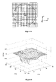
- FIG. 6 a shows the 30-mm diameter, 2 mm ⁇ 2 mm sampling grid, circular pupil without central obstruction shown within the extended domain ⁇ 1 .
- FIG. 6 b shows the ground-truth wavefront within the 30-mm diameter circular pupil without central obstruction on a vertical scale of ⁇ 1 ⁇ m.
- FIG. 8 a shows a 30-mm diameter circular pupil with a 10% central obstruction.
- FIG. 8 b shows the ground-truth wavefront for a 30-mm diameter circular pupil with a 10% central obstruction on a vertical scale of ⁇ 1 ⁇ m.
- FIG. 10 shows a plot of RMS deviation errors in units of wavelength as a function of the number of iterations for the two data sets considered.
- FIG. 11 shows the noise coefficient limit versus the dimension size of the sampling grid.
- FIG. 12 shows the normal matrix condition number versus grid dimension size.
- the Southwell geometry is characterized by taking the wavefront slope measurements and wavefront values estimation at the same nodes.
- FIG. 2 shows the geometry in the y-direction with both the wavefront nodes i and the interlaced nodes j.
- the slope data between two adjacent nodes was assumed to change linearly with distance, which allows linear interpolation to estimate the slopes between nodes.
- the slope at node j was then estimated as an average of the slopes at nodes i and i+1 by:
- s yj 1 2 ⁇ ( s y i + s y i + 1 ) , ( 1 ) where the slope s yj could also be expressed as the difference quotient of the wavefront values at nodes i and i+1 to their separation a, so that
- Equations (3) and (4) may be written in matrix form as:
- the present invention expands on the method of Zou et al. and presents an iterative procedure to improve the accuracy of the final wavefront estimation within the measured pupil.
- the merit of the iterative procedure is that it yields negligible RMS deviation errors while it still provides a universal reconstruction matrix for any irregular pupil shape and size.
- all the matrix coefficients are determined and known once and for all.
- the matrix is sparse, symmetrical, and regular and the matrix elements can be expressed as a function of the matrix index using the Kronecker's delta function.
- the algorithm detailed hereafter will first require calculating slope data from the estimated wavefront in order to enable the iterative process. Such computations will be first presented.
- Slope computation from a known wavefront may be thought simply as the inverse problem of wavefront estimation from slope data.
- the equations established by Zou et al. can be inverted to obtain a matrix equation set for slope extraction.
- the matrix developed out of these reversed equations is rank-deficient for estimating the slope data from the reconstructed wavefront.
- Such a finding is intrinsically linked to the Southwell geometry chosen for the problem.
- additional independent equations are required.
- Such equations will be based on curvature estimates, and the equations for slope computation will thus be grouped into two types: slope-based and curvature-based.
- the matrix for extracting the y-direction slopes will first be described.
- the matrix for extracting the z-direction slopes will then be provided.
- Equation (12) is divided by the grid separation a, it will actually be a discrete approximation of wavefront curvature at node j+1, which is of O(a 3 ) precision as shown in Equation (A12).
- Equation (A14) The derivation of Equation (27) is shown by Equation (A14).
- V [ G H ] , ( 32 ) and
- Equation (7) the wavefront is reconstructed from slope data in ⁇ 1 410 .
- the matrix equation sets given by Equations (22) and (36) are used to compute they and z slopes in ⁇ 1 from the reconstructed wavefront 440 .
- the computed slopes 450 are compared with the original slope data within ⁇ 0 460 . If the differences are negligible (i.e. less than a termination criterion) 470 , the reconstructed wavefront over ⁇ 1 is output 480 , among which only the wavefront within ⁇ 0 is of interest. Otherwise, the slope data in ⁇ 0 are replaced with the original measured slope data 430 , while the slope data in the extended area ⁇ 1 ⁇ 0 are kept unchanged. The iterative process continues until it satisfies the established termination criterion.
- Such iterative processes are referred to as the Gerchberg-type iterations, because the iterative process bears analogy to the Gerchberg-Saxton algorithm, which consists in substituting the computed amplitude of a discrete complex function in the pupil under test with the sampled amplitude across iterations, until both amplitude and phase converged to a solution.
- the iterative algorithm presented in this invention substitutes the slope data in the pupil under test with the sampled raw slope data iteratively until the reconstructed wavefront converges to a unique solution.
- the Gerchberg-Saxton iterations were based on Fourier transforms, while the algorithm detailed in this invention is based on the linear LS method.
- Roddier et al. The algorithm disclosed here bears similarity to that taught by Roddier et al. in the sense that both algorithms use Gerchberg-type iterations to extrapolate the wavefront outside of the boundary.
- a basic difference is that Roddier et al. algorithm is based on FFTs instead of the linear LS method.
- the slope data inside the pupil under test are from wavefront measurements, and the slopes outside of the pupil under test are zero. Therefore, the slope data crossing the original pupil boundaries between ⁇ 0 and ⁇ 1 ⁇ 0 are not continuous, and such discontinuous boundary conditions yield severe errors in the reconstructed wavefront not only at the edge of the pupil, but also within the pupil of interest through propagation of errors. In other words, when the slopes do not satisfy the derivative continuity condition of the Poisson equation, deviation errors will be induced.
- FIG. 5 a shows an example of an original wavefront (i.e. a reconstructed wavefront which is considered to represent ground truth of wavefront reconstruction as will be further explained below), while the estimated wavefront from slope data without iterations is shown in FIG. 5 b.
- an original wavefront i.e. a reconstructed wavefront which is considered to represent ground truth of wavefront reconstruction as will be further explained below
- the estimated wavefront from slope data without iterations is shown in FIG. 5 b.
- the differences between the estimated and the original wavefronts represent the deviation errors associated with the domain extension of Zou et al. Therefore, while the domain extension technique is quite useful for developing a universal algorithm, provided that the extended wavefront reconstruction matrix is universal and regular to accommodate irregular pupil shapes and enables efficient computations, the challenge lies in how to establish continuity constraints at the boundaries between ⁇ 0 and ⁇ 1 ⁇ 0 to remove the deviation errors in the estimated wavefront.
- the iterative process enables a continuous practical extrapolation of the slope data outside of the optical pupil ⁇ 0 , while it does not interfere with the internal region of ⁇ 0 .
- the iterative algorithm converges quickly to an unbiased solution, while at the same time the smoother the wavefront surface under construction, the smaller the residue deviation error as expected, and the fewer iterations needed. Theoretically, the deviation error of this unique solution will decrease to zero. However, measurement noise prohibits the deviation errors from reaching zero, so they stagger to its minimum.
- the gradient-based iterative wavefront estimation algorithm presented in the present invention finds applications to regularly- and irregularly-shaped pupils.
- two examples are presented, one with a circular 30-mm diameter pupil, and another with the same size pupil but with a 10% central obstruction. Both data sets were acquired from a previous experiment reported by Zou et al.
- the obstructed wavefront was obtained by considering the slope data within the obstructed pupil only.
- the wavefronts were reconstructed without the domain extension technique from the same set of slope data with the conventional iterative or direct methods, such as the Jacobi iterative method, the Gauss elimination method, and the Cholesky decomposition method.
- a circular pupil without obstruction is a simply connected domain.
- the considered 30-mm diameter pupil with an array of 161 Shack-Hartmann grid points is shown in FIG. 6 a .
- the points outside of the circular pupil in the square lattice are the imaginary grid points.
- the ground-truth wavefront is also shown in FIG. 6 b .
- the 30-mm circular pupil with a 10% central obstruction is shown in FIG. 8 a .
- Such a percent of obscuration is common for astronomical telescope mirrors.
- an algorithm that enables testing of any pupil shape without any additional steps in preparing and setting-up for such test provides key advantages not only in time efficiency but also in minimizing the risk of test-induced errors.
- the ground-truth wavefront is shown in FIG. 8 b.
- Deviation-error maps of the wavefronts reconstructed by the Gerchberg-type iterative algorithm with several numbers of iterations are shown in FIGS. 9 a – 9 f .
- the algorithmic convergence for the present invention is superior to the prior arts.
- the deviation error reduction through Gerchberg-type iterations was found to be efficient. Specifically, the final deviation errors after a maximum of 5 iterations for the two examples considered were less than ⁇ /100 for ⁇ equal to 632.8 nm, as shown in FIGS. 7 a – 7 f and FIGS. 9 a – 9 f .
- the convergence indicated by the RMS wavefront error in units of wavelength as a function of the number of iterations is plotted in FIG. 10 for the two case datasets presented above. Such a finding is high performance for optical testing, and the algorithm can be said to be very efficient.
- the fill-in factor of the wavefront reconstruction matrix C T C is (5t ⁇ 4)/t 3
- the fill-in factors of the slope computation matrices A T A and B T B are both(t+4)/t 3 .
- FLOPS Floating-Point Operations
- the positive definite slope-extraction matrices A T A and B T B are banded and diagonal with semi-bandwidths of 2 and t, respectively.
- a direct solution method such as the Cholesky method to solve the normal equation sets because the matrices A T A and B T B can be decomposed into two unique triangular matrices by simple derivations once and for all. Thereby no more Cholesky decompositions are needed in computation.
- the computations needed in solving the two systems of equations are substitutions only, which need arithmetic costs of about 4m times the bandwidth, which yields 8t 2 FLOPS for A T A and 4t 3 FLOPS for B T B.
- the computational cost needed for substitutions in solving an equation without exploiting the band structure is 2t 4 FLOPS.
- the zero-point for the wavefront under construction is set to make the matrix C T C positive definite before the Cholesky decomposition is performed. Since it is a banded sparse matrix with a semi-bandwidth of t, this equation set can be solved by a banded Cholesky decomposition method, which needs about t 4 FLOPS for decomposition and 4t 3 FLOPS for substitutions. As a comparison, employing the conventional Cholesky method to solve this equation set without exploiting the band structure of the matrix yields approximately
- the SVD method needs about 12t 6 FLOPS. Because the SVD method yields a unique solution with minimum-norm for a rank deficient least squares problem, it is a good method in practice if the computational complexity is not a constraint.
- SOR Successive Over-Relaxation
- the computational cost needed for solving Equation (7) with the optimal SOR method is approximately 15t 3 FLOPS.
- the analysis indicates that the banded Cholesky method needs less FLOPS of computational cost for a small grid size (t ⁇ 11), but for a large grid size the SOR method is computationally less expensive.
- the complexity of the optimal SOR method increases with a cubic curve, whereas the complexity of banded Cholesky method increases with a quadratic curve.
- the complexity of the present invention is now compared with the complexity of FFT-based iterative algorithms.
- the FFT-based iterative algorithm proposed by Roddier et al. needs to compute two FFTs besides the computations of the y- and the z-slopes from the wavefront at each iteration.
- the FFT-based algorithms usually converge slowly; for example, the Gerchberg-Saxton algorithm needs at least tens to hundreds or even thousands of iterations to converge to a solution, while the algorithm of the present invention converges to less than ⁇ /100 deviation error after a maximum of approximately five iterations.
- the error propagation coefficient of the present invention is slow as compared to the prior art. If the perturbations introduced by the rounding errors are neglected, wavefront errors may occur from two sources: the algorithm discretization errors that depend on the basic reconstruction scheme adopted, and the wavefront sensor measurement error, such as the CCD centroiding.
- the discretization errors of the wavefront reconstruction scheme adopted by this invention have been discussed by Zou et al.
- the error propagation of the wavefront reconstruction from the wavefront measurements is now considered.
- the noise coefficient is defined as taught by Southwell.
- a universal wavefront reconstruction matrix C is assumed.
- the Euclidian norm of vector X is introduced as
- ⁇ X ⁇ 2 ( X T ⁇ X ) 1 / 2 , ( 39 ) and the corresponding matrix norm for a matrix C as
- Equation (41) becomes
- ⁇ w and ⁇ s are the rms errors of the wavefront and the wavefront slope measurements, respectively.
- Equation (50) points to the well-known fact that the error propagation coefficient is limited by the reciprocal of the minimum eigenvalue of the normal matrix.
- Equations (22) and (36) The analysis is also applicable to the error propagation of slope computation provided by Equations (22) and (36).
- the problem is then reduced to evaluating the minimum eigenvalue of the normal matrix. Since the normal equation matrix is symmetric, the classical Jacobi method can be employed to compute the eigenvalues.
- Equation (7) For the wavefront reconstruction matrix in Equation (7), the situation is more complex because the eigenvalues of this matrix are sensitive to the variation of the wavefront zero-point, the matrix dimension size, and even the parity of the number of the matrix dimension.
- the curve of the noise coefficient limit versus the grid size of the wavefront is obtained and shown in FIG. 11 . Results show that the wavefront reconstruction has a better performance in error propagation when the number of the reconstruction matrix dimension is odd. Therefore, an odd number of the sampling grid array is preferable to its closest even number of the sampling grid array. Making a least square fitting of this curve, the relationship can be expressed quantitatively as
- ⁇ w 2 / ⁇ d 2 ⁇ ⁇ 2 ⁇ ⁇ - 44 + 28.577 ⁇ e t 8.925 , t ⁇ ⁇ is ⁇ ⁇ even - 31.875 + 20.607 ⁇ e t 7.766 , t ⁇ ⁇ is ⁇ ⁇ odd ⁇ ( 52 )
- w i w i + 1 2 - a 2 ⁇ ⁇ W ⁇ y ⁇ i + 1 2 + a 2 4 ⁇ 2 ! ⁇ ⁇ 2 ⁇ W ⁇ y 2 ⁇ i + 1 2 - a 3 8 ⁇ 3 ! ⁇ ⁇ 3 ⁇ W ⁇ y 3 ⁇ i + 1 2 + a 4 16 ⁇ 4 ! ⁇ ⁇ 4 ⁇ W ⁇ y 4 ⁇ i + 1 2 + O ⁇ ( a 5 ) , ⁇ ( A1 ) and
- Equation (A3) may be expressed as
- a wavefront reconstruction algorithm suitable for practical use must have the following properties: (a) the wavefront estimates must be unbiased; (b) the error propagation coefficient must be slow; (c) the computation must be efficient, especially for large datasets, and the necessary memory space should be small enough to be applicable in the laboratory; finally, (d) the algorithm should be easily adaptable to various pupil shapes.
- a Gerchberg-Saxton type iterative process was combined with a linear least-squares method to obtain a practical unbiased wavefront estimation algorithm that combines the accuracy of the iterative wavefront extrapolation technique with the linear sparse matrix efficiency.
- This invention has applications in such diverse fields as ophthalmometry, optical astronomy, laser beam profiling, optical component testing, and microscopy.
- This invention is particularly applicable in the field of adaptive optics in which the components of an optical system are actively manipulated to maintain high image quality.
- the resolution of ground-based telescopes is highly dependent on the amount of atmospheric turbulence present, as this causes distortion of the wavefront and thus a reduction in image quality.
- atmospheric distortion is measured by a wavefront sensor which then provides a control signal based on the reconstructed wavefront for corrective optics such as deformable mirrors.
- Such a system typically has to work at speeds sufficient to keep up with the rapid atmospheric changes.
- wavefront sensing and reconstruction is increasingly being used to characterize higher-order aberrations in the human eye, providing vital information for corrective eye surgery.
- Wavefront sensing and reconstruction also has application in testing individual optical components, such as mirrors and lenses.
- the information obtained from a reconstructed wavefront can lead to reduced development times, reduced component cost, and improved optical performance.
Abstract
Description
where the slope syj could also be expressed as the difference quotient of the wavefront values at nodes i and i+1 to their separation a, so that
By combining Equations (1) and (2), a relationship between the wavefront slopes and the wavefront values at i+1 and i was established as
Similarly in the z direction and accounting for the sign convention shown in
-
- 1. Without loss of generality, assume that the regular square net has t×t=m grid points.
- 2. The original sampling domain Ω0 (i.e. exit pupil, simply connected domain or multiple connected domains) was embedded into a regular square domain Ω1 that contains the sampling domain Ω0. Then the square domain Ω1 was thought of being composed of two parts: the real part Ω0 and the imaginary part Ω1\Ω0, as shown in
FIG. 3 . - 3. The grid points in Ω1 were indexed sequentially from 1 to m row by row (the grid points could also be indexed equivalently column by column as an alternative).
- 4. The slopes were set to zero in the imaginary part Ω1\Ω0.
or
CW=S, (5b)
where Ci+1,i and di+1,i are defined as
C T CW=C T S. (7)
s yi+1 +s yi =e j, (8)
where
A 1 S y =E, (10)
which is not a full-rank matrix equation set. Curvature-based equations are then considered to determine a unique solution for slope extraction. The curvature at a midpoint node j+1 is proportional to the slope difference between adjacent points i+1 and i+2. According to
s yi+2 −s yi+1 =f j+1, (11)
where
A 2 S y =F. (13)
A S y =U, (14)
where
S y =[s y1 s y2 . . . s ym]T, (16)
with
A 1=diag[D 1 ,D 1 , . . . ,D 1]ε, (18)
A 2=diag[D2 ,D 2 , . . . ,D 2]ε, (19)
where
and
A T AS y =A T U. (22)
s z,i +s z,i+1 =g j , i=1, 2, . . . ,m−t, (23)
where
In matrix form, Equation (23) may be written as
B 1 S z =G (25)
which is not a full-rank matrix equation. To get a full-rank equation set, we add the curvature-based equations
s z,i+t −s z,i+2 t=h j+t, (26)
where
and i=1,2, . . . t; t+1, t+2, . . . 2t−3, . . . , m−3t. The derivation of Equation (27) is shown by Equation (A14).
B 2 S z =H. (28)
Combining Eqs. (25) and (28) in a matrix-form equation set, we obtain
BS z =V, (29)
s z [s z1 s z2 . . . s zm]T (31)
and
B T BS z =B TV. (36)
Gerchberg-Type Iterative Wavefront Estimation Algorithm
FLOPS.
FLOPS, and the SVD method needs about 12t6 FLOPS. Because the SVD method yields a unique solution with minimum-norm for a rank deficient least squares problem, it is a good method in practice if the computational complexity is not a constraint.
C T CW′=aC T S′ (38)
where C was defined in Equation (5), and a is the distance between grid points. The Euclidian norm of vector X is introduced as
and the corresponding matrix norm for a matrix C as
where ρ(CTC) is the spectral radius of CTC. If CTC is invertible, then
where cond(CTC) is defined as the matrix condition number of CTC, and
cond(C T C):=lub2 (C T C) lub2[(C T C)−1]=ρ(C T C)ρ[(C T C)−1]. (42)
and
where σw and σs are the rms errors of the wavefront and the wavefront slope measurements, respectively. According to Equations (44)–(46)
σw≦γσd, (48)
where
γ=|λmin|−1/2. (49)
σw 2/σd 2≦γ2−|λmin|−1. (50)
as the n′th derivative of the wavefront at point i, and
as the n′th derivative of the wavefront at the midpoint between the points i and i+1. According to Taylor's series
and
By subtracting Equation (A1) from (A2),
By adding Equation (A1) to (A2),
The replacement of w with
yields
And using Equation (A6), Equation (A3) may be expressed as
Again, replace w with
now in Equation (A7), to yield
and
where
Combining Eq. (A10) and Eq. (A8)
or
where i=1,2, . . . t−3; t+1,t+2, . . . 2t−3, . . . m−3.
Similarly in the z-direction,
where i=1,2, . . . t, t+1,t+2, . . . 2t, . . . , m−3t.
Claims (14)
Priority Applications (1)
| Application Number | Priority Date | Filing Date | Title |
|---|---|---|---|
| US10/867,527 US7088457B1 (en) | 2003-10-01 | 2004-06-10 | Iterative least-squares wavefront estimation for general pupil shapes |
Applications Claiming Priority (2)
| Application Number | Priority Date | Filing Date | Title |
|---|---|---|---|
| US50765703P | 2003-10-01 | 2003-10-01 | |
| US10/867,527 US7088457B1 (en) | 2003-10-01 | 2004-06-10 | Iterative least-squares wavefront estimation for general pupil shapes |
Publications (1)
| Publication Number | Publication Date |
|---|---|
| US7088457B1 true US7088457B1 (en) | 2006-08-08 |
Family
ID=36942017
Family Applications (1)
| Application Number | Title | Priority Date | Filing Date |
|---|---|---|---|
| US10/867,527 Active 2025-02-19 US7088457B1 (en) | 2003-10-01 | 2004-06-10 | Iterative least-squares wavefront estimation for general pupil shapes |
Country Status (1)
| Country | Link |
|---|---|
| US (1) | US7088457B1 (en) |
Cited By (46)
| Publication number | Priority date | Publication date | Assignee | Title |
|---|---|---|---|---|
| US20080077644A1 (en) * | 2006-07-10 | 2008-03-27 | Visx, Incorporated | Systems and methods for wavefront analysis over circular and noncircular pupils |
| US20100256967A1 (en) * | 2009-04-02 | 2010-10-07 | United States Of America As Represented By The Administrator Of The National Aeronautics And Spac | Variable sample mapping algorithm |
| US20120321219A1 (en) * | 2011-06-15 | 2012-12-20 | Keithley Douglas G | Modified bicubic interpolation |
| US20120327287A1 (en) * | 2007-12-06 | 2012-12-27 | U.S. Government As Represented By The Secretary Of The Army | Method and system for producing image frames using quantum properties |
| CN107833251A (en) * | 2017-11-13 | 2018-03-23 | 京东方科技集团股份有限公司 | Pupil positioning device and method, the display driver of virtual reality device |
| US10089516B2 (en) | 2013-07-31 | 2018-10-02 | Digilens, Inc. | Method and apparatus for contact image sensing |
| US10145533B2 (en) | 2005-11-11 | 2018-12-04 | Digilens, Inc. | Compact holographic illumination device |
| US10156681B2 (en) | 2015-02-12 | 2018-12-18 | Digilens Inc. | Waveguide grating device |
| US10185154B2 (en) | 2011-04-07 | 2019-01-22 | Digilens, Inc. | Laser despeckler based on angular diversity |
| US10209517B2 (en) | 2013-05-20 | 2019-02-19 | Digilens, Inc. | Holographic waveguide eye tracker |
| US10216061B2 (en) | 2012-01-06 | 2019-02-26 | Digilens, Inc. | Contact image sensor using switchable bragg gratings |
| US10234696B2 (en) | 2007-07-26 | 2019-03-19 | Digilens, Inc. | Optical apparatus for recording a holographic device and method of recording |
| US10241330B2 (en) | 2014-09-19 | 2019-03-26 | Digilens, Inc. | Method and apparatus for generating input images for holographic waveguide displays |
| US10330777B2 (en) | 2015-01-20 | 2019-06-25 | Digilens Inc. | Holographic waveguide lidar |
| US10359736B2 (en) | 2014-08-08 | 2019-07-23 | Digilens Inc. | Method for holographic mastering and replication |
| US10423222B2 (en) | 2014-09-26 | 2019-09-24 | Digilens Inc. | Holographic waveguide optical tracker |
| US10437051B2 (en) | 2012-05-11 | 2019-10-08 | Digilens Inc. | Apparatus for eye tracking |
| US10437064B2 (en) | 2015-01-12 | 2019-10-08 | Digilens Inc. | Environmentally isolated waveguide display |
| US10459145B2 (en) | 2015-03-16 | 2019-10-29 | Digilens Inc. | Waveguide device incorporating a light pipe |
| US10545346B2 (en) | 2017-01-05 | 2020-01-28 | Digilens Inc. | Wearable heads up displays |
| US10591756B2 (en) | 2015-03-31 | 2020-03-17 | Digilens Inc. | Method and apparatus for contact image sensing |
| US10642058B2 (en) | 2011-08-24 | 2020-05-05 | Digilens Inc. | Wearable data display |
| US10670876B2 (en) | 2011-08-24 | 2020-06-02 | Digilens Inc. | Waveguide laser illuminator incorporating a despeckler |
| US10678053B2 (en) | 2009-04-27 | 2020-06-09 | Digilens Inc. | Diffractive projection apparatus |
| US10690916B2 (en) | 2015-10-05 | 2020-06-23 | Digilens Inc. | Apparatus for providing waveguide displays with two-dimensional pupil expansion |
| US10690851B2 (en) | 2018-03-16 | 2020-06-23 | Digilens Inc. | Holographic waveguides incorporating birefringence control and methods for their fabrication |
| US10732569B2 (en) | 2018-01-08 | 2020-08-04 | Digilens Inc. | Systems and methods for high-throughput recording of holographic gratings in waveguide cells |
| US10859768B2 (en) | 2016-03-24 | 2020-12-08 | Digilens Inc. | Method and apparatus for providing a polarization selective holographic waveguide device |
| US10890707B2 (en) | 2016-04-11 | 2021-01-12 | Digilens Inc. | Holographic waveguide apparatus for structured light projection |
| US10914950B2 (en) | 2018-01-08 | 2021-02-09 | Digilens Inc. | Waveguide architectures and related methods of manufacturing |
| US10942430B2 (en) | 2017-10-16 | 2021-03-09 | Digilens Inc. | Systems and methods for multiplying the image resolution of a pixelated display |
| US10983340B2 (en) | 2016-02-04 | 2021-04-20 | Digilens Inc. | Holographic waveguide optical tracker |
| CN113343163A (en) * | 2021-04-19 | 2021-09-03 | 华南农业大学 | Large-scale corner mesh adjustment and precision evaluation method, system and storage medium |
| US20210311225A1 (en) * | 2018-11-13 | 2021-10-07 | Mitsubishi Heavy Industries, Ltd. | Optical system and optical compensation method |
| US11307432B2 (en) | 2014-08-08 | 2022-04-19 | Digilens Inc. | Waveguide laser illuminator incorporating a Despeckler |
| US11378732B2 (en) | 2019-03-12 | 2022-07-05 | DigLens Inc. | Holographic waveguide backlight and related methods of manufacturing |
| US11402801B2 (en) | 2018-07-25 | 2022-08-02 | Digilens Inc. | Systems and methods for fabricating a multilayer optical structure |
| US11442222B2 (en) | 2019-08-29 | 2022-09-13 | Digilens Inc. | Evacuated gratings and methods of manufacturing |
| US11448937B2 (en) | 2012-11-16 | 2022-09-20 | Digilens Inc. | Transparent waveguide display for tiling a display having plural optical powers using overlapping and offset FOV tiles |
| US11460621B2 (en) | 2012-04-25 | 2022-10-04 | Rockwell Collins, Inc. | Holographic wide angle display |
| US11480788B2 (en) | 2015-01-12 | 2022-10-25 | Digilens Inc. | Light field displays incorporating holographic waveguides |
| US11513350B2 (en) | 2016-12-02 | 2022-11-29 | Digilens Inc. | Waveguide device with uniform output illumination |
| US11543594B2 (en) | 2019-02-15 | 2023-01-03 | Digilens Inc. | Methods and apparatuses for providing a holographic waveguide display using integrated gratings |
| US11681143B2 (en) | 2019-07-29 | 2023-06-20 | Digilens Inc. | Methods and apparatus for multiplying the image resolution and field-of-view of a pixelated display |
| US11726332B2 (en) | 2009-04-27 | 2023-08-15 | Digilens Inc. | Diffractive projection apparatus |
| US11747568B2 (en) | 2019-06-07 | 2023-09-05 | Digilens Inc. | Waveguides incorporating transmissive and reflective gratings and related methods of manufacturing |
Citations (6)
| Publication number | Priority date | Publication date | Assignee | Title |
|---|---|---|---|---|
| US4804269A (en) * | 1987-08-11 | 1989-02-14 | Litton Systems, Inc. | Iterative wavefront measuring device |
| US5864381A (en) * | 1996-07-10 | 1999-01-26 | Sandia Corporation | Automated pupil remapping with binary optics |
| US6184974B1 (en) * | 1999-07-01 | 2001-02-06 | Wavefront Sciences, Inc. | Apparatus and method for evaluating a target larger than a measuring aperture of a sensor |
| US20040130705A1 (en) * | 2002-07-09 | 2004-07-08 | Topa Daniel M. | System and method of wavefront sensing |
| US6956657B2 (en) * | 2001-12-18 | 2005-10-18 | Qed Technologies, Inc. | Method for self-calibrated sub-aperture stitching for surface figure measurement |
| US20060071155A1 (en) * | 2004-01-08 | 2006-04-06 | Equus Inc. | Safety device for garage door |
-
2004
- 2004-06-10 US US10/867,527 patent/US7088457B1/en active Active
Patent Citations (6)
| Publication number | Priority date | Publication date | Assignee | Title |
|---|---|---|---|---|
| US4804269A (en) * | 1987-08-11 | 1989-02-14 | Litton Systems, Inc. | Iterative wavefront measuring device |
| US5864381A (en) * | 1996-07-10 | 1999-01-26 | Sandia Corporation | Automated pupil remapping with binary optics |
| US6184974B1 (en) * | 1999-07-01 | 2001-02-06 | Wavefront Sciences, Inc. | Apparatus and method for evaluating a target larger than a measuring aperture of a sensor |
| US6956657B2 (en) * | 2001-12-18 | 2005-10-18 | Qed Technologies, Inc. | Method for self-calibrated sub-aperture stitching for surface figure measurement |
| US20040130705A1 (en) * | 2002-07-09 | 2004-07-08 | Topa Daniel M. | System and method of wavefront sensing |
| US20060071155A1 (en) * | 2004-01-08 | 2006-04-06 | Equus Inc. | Safety device for garage door |
Non-Patent Citations (1)
| Title |
|---|
| Zou and Zhang, Generalized Wave-Front Reconstruction Algorithm Applied in a Shack-Hartmann Test, Jan. 10, 2000, p. 250-268, Applied Optics/vol. 39, No. 2. |
Cited By (78)
| Publication number | Priority date | Publication date | Assignee | Title |
|---|---|---|---|---|
| US10145533B2 (en) | 2005-11-11 | 2018-12-04 | Digilens, Inc. | Compact holographic illumination device |
| US8504329B2 (en) * | 2006-07-10 | 2013-08-06 | Amo Manufacturing Usa, Llc. | Systems and methods for wavefront analysis over circular and noncircular pupils |
| US8983812B2 (en) | 2006-07-10 | 2015-03-17 | Amo Development, Llc | Systems and methods for wavefront analysis over circular and noncircular pupils |
| US20080077644A1 (en) * | 2006-07-10 | 2008-03-27 | Visx, Incorporated | Systems and methods for wavefront analysis over circular and noncircular pupils |
| US10234696B2 (en) | 2007-07-26 | 2019-03-19 | Digilens, Inc. | Optical apparatus for recording a holographic device and method of recording |
| US10725312B2 (en) | 2007-07-26 | 2020-07-28 | Digilens Inc. | Laser illumination device |
| US20120327287A1 (en) * | 2007-12-06 | 2012-12-27 | U.S. Government As Represented By The Secretary Of The Army | Method and system for producing image frames using quantum properties |
| US8811763B2 (en) * | 2007-12-06 | 2014-08-19 | The United States Of America As Represented By The Secretary Of The Army | Method and system for producing image frames using quantum properties |
| US20100256967A1 (en) * | 2009-04-02 | 2010-10-07 | United States Of America As Represented By The Administrator Of The National Aeronautics And Spac | Variable sample mapping algorithm |
| US10678053B2 (en) | 2009-04-27 | 2020-06-09 | Digilens Inc. | Diffractive projection apparatus |
| US11175512B2 (en) | 2009-04-27 | 2021-11-16 | Digilens Inc. | Diffractive projection apparatus |
| US11726332B2 (en) | 2009-04-27 | 2023-08-15 | Digilens Inc. | Diffractive projection apparatus |
| US11487131B2 (en) | 2011-04-07 | 2022-11-01 | Digilens Inc. | Laser despeckler based on angular diversity |
| US10185154B2 (en) | 2011-04-07 | 2019-01-22 | Digilens, Inc. | Laser despeckler based on angular diversity |
| US8953907B2 (en) * | 2011-06-15 | 2015-02-10 | Marvell World Trade Ltd. | Modified bicubic interpolation |
| US20120321219A1 (en) * | 2011-06-15 | 2012-12-20 | Keithley Douglas G | Modified bicubic interpolation |
| US9563935B2 (en) | 2011-06-15 | 2017-02-07 | Marvell World Trade Ltd. | Modified bicubic interpolation |
| US10670876B2 (en) | 2011-08-24 | 2020-06-02 | Digilens Inc. | Waveguide laser illuminator incorporating a despeckler |
| US10642058B2 (en) | 2011-08-24 | 2020-05-05 | Digilens Inc. | Wearable data display |
| US11287666B2 (en) | 2011-08-24 | 2022-03-29 | Digilens, Inc. | Wearable data display |
| US10216061B2 (en) | 2012-01-06 | 2019-02-26 | Digilens, Inc. | Contact image sensor using switchable bragg gratings |
| US10459311B2 (en) | 2012-01-06 | 2019-10-29 | Digilens Inc. | Contact image sensor using switchable Bragg gratings |
| US11460621B2 (en) | 2012-04-25 | 2022-10-04 | Rockwell Collins, Inc. | Holographic wide angle display |
| US10437051B2 (en) | 2012-05-11 | 2019-10-08 | Digilens Inc. | Apparatus for eye tracking |
| US11448937B2 (en) | 2012-11-16 | 2022-09-20 | Digilens Inc. | Transparent waveguide display for tiling a display having plural optical powers using overlapping and offset FOV tiles |
| US11815781B2 (en) * | 2012-11-16 | 2023-11-14 | Rockwell Collins, Inc. | Transparent waveguide display |
| US20230114549A1 (en) * | 2012-11-16 | 2023-04-13 | Rockwell Collins, Inc. | Transparent waveguide display |
| US11662590B2 (en) | 2013-05-20 | 2023-05-30 | Digilens Inc. | Holographic waveguide eye tracker |
| US10209517B2 (en) | 2013-05-20 | 2019-02-19 | Digilens, Inc. | Holographic waveguide eye tracker |
| US10423813B2 (en) | 2013-07-31 | 2019-09-24 | Digilens Inc. | Method and apparatus for contact image sensing |
| US10089516B2 (en) | 2013-07-31 | 2018-10-02 | Digilens, Inc. | Method and apparatus for contact image sensing |
| US11709373B2 (en) | 2014-08-08 | 2023-07-25 | Digilens Inc. | Waveguide laser illuminator incorporating a despeckler |
| US10359736B2 (en) | 2014-08-08 | 2019-07-23 | Digilens Inc. | Method for holographic mastering and replication |
| US11307432B2 (en) | 2014-08-08 | 2022-04-19 | Digilens Inc. | Waveguide laser illuminator incorporating a Despeckler |
| US10241330B2 (en) | 2014-09-19 | 2019-03-26 | Digilens, Inc. | Method and apparatus for generating input images for holographic waveguide displays |
| US11726323B2 (en) | 2014-09-19 | 2023-08-15 | Digilens Inc. | Method and apparatus for generating input images for holographic waveguide displays |
| US10423222B2 (en) | 2014-09-26 | 2019-09-24 | Digilens Inc. | Holographic waveguide optical tracker |
| US11480788B2 (en) | 2015-01-12 | 2022-10-25 | Digilens Inc. | Light field displays incorporating holographic waveguides |
| US11740472B2 (en) | 2015-01-12 | 2023-08-29 | Digilens Inc. | Environmentally isolated waveguide display |
| US11726329B2 (en) | 2015-01-12 | 2023-08-15 | Digilens Inc. | Environmentally isolated waveguide display |
| US10437064B2 (en) | 2015-01-12 | 2019-10-08 | Digilens Inc. | Environmentally isolated waveguide display |
| US10330777B2 (en) | 2015-01-20 | 2019-06-25 | Digilens Inc. | Holographic waveguide lidar |
| US10156681B2 (en) | 2015-02-12 | 2018-12-18 | Digilens Inc. | Waveguide grating device |
| US11703645B2 (en) | 2015-02-12 | 2023-07-18 | Digilens Inc. | Waveguide grating device |
| US10527797B2 (en) | 2015-02-12 | 2020-01-07 | Digilens Inc. | Waveguide grating device |
| US10459145B2 (en) | 2015-03-16 | 2019-10-29 | Digilens Inc. | Waveguide device incorporating a light pipe |
| US10591756B2 (en) | 2015-03-31 | 2020-03-17 | Digilens Inc. | Method and apparatus for contact image sensing |
| US11281013B2 (en) | 2015-10-05 | 2022-03-22 | Digilens Inc. | Apparatus for providing waveguide displays with two-dimensional pupil expansion |
| US10690916B2 (en) | 2015-10-05 | 2020-06-23 | Digilens Inc. | Apparatus for providing waveguide displays with two-dimensional pupil expansion |
| US11754842B2 (en) | 2015-10-05 | 2023-09-12 | Digilens Inc. | Apparatus for providing waveguide displays with two-dimensional pupil expansion |
| US10983340B2 (en) | 2016-02-04 | 2021-04-20 | Digilens Inc. | Holographic waveguide optical tracker |
| US11604314B2 (en) | 2016-03-24 | 2023-03-14 | Digilens Inc. | Method and apparatus for providing a polarization selective holographic waveguide device |
| US10859768B2 (en) | 2016-03-24 | 2020-12-08 | Digilens Inc. | Method and apparatus for providing a polarization selective holographic waveguide device |
| US10890707B2 (en) | 2016-04-11 | 2021-01-12 | Digilens Inc. | Holographic waveguide apparatus for structured light projection |
| US11513350B2 (en) | 2016-12-02 | 2022-11-29 | Digilens Inc. | Waveguide device with uniform output illumination |
| US11194162B2 (en) | 2017-01-05 | 2021-12-07 | Digilens Inc. | Wearable heads up displays |
| US10545346B2 (en) | 2017-01-05 | 2020-01-28 | Digilens Inc. | Wearable heads up displays |
| US11586046B2 (en) | 2017-01-05 | 2023-02-21 | Digilens Inc. | Wearable heads up displays |
| US10942430B2 (en) | 2017-10-16 | 2021-03-09 | Digilens Inc. | Systems and methods for multiplying the image resolution of a pixelated display |
| CN107833251A (en) * | 2017-11-13 | 2018-03-23 | 京东方科技集团股份有限公司 | Pupil positioning device and method, the display driver of virtual reality device |
| US10699117B2 (en) | 2017-11-13 | 2020-06-30 | Boe Technology Group Co., Ltd. | Pupil positioning device and method and display driver of virtual reality device |
| CN107833251B (en) * | 2017-11-13 | 2020-12-04 | 京东方科技集团股份有限公司 | Pupil positioning device and method and display driver of virtual reality equipment |
| US10914950B2 (en) | 2018-01-08 | 2021-02-09 | Digilens Inc. | Waveguide architectures and related methods of manufacturing |
| US10732569B2 (en) | 2018-01-08 | 2020-08-04 | Digilens Inc. | Systems and methods for high-throughput recording of holographic gratings in waveguide cells |
| US11150408B2 (en) | 2018-03-16 | 2021-10-19 | Digilens Inc. | Holographic waveguides incorporating birefringence control and methods for their fabrication |
| US10690851B2 (en) | 2018-03-16 | 2020-06-23 | Digilens Inc. | Holographic waveguides incorporating birefringence control and methods for their fabrication |
| US11726261B2 (en) | 2018-03-16 | 2023-08-15 | Digilens Inc. | Holographic waveguides incorporating birefringence control and methods for their fabrication |
| US11402801B2 (en) | 2018-07-25 | 2022-08-02 | Digilens Inc. | Systems and methods for fabricating a multilayer optical structure |
| US20210311225A1 (en) * | 2018-11-13 | 2021-10-07 | Mitsubishi Heavy Industries, Ltd. | Optical system and optical compensation method |
| US11802990B2 (en) * | 2018-11-13 | 2023-10-31 | Mitsubishi Heavy Industries, Ltd. | Optical system and optical compensation method |
| US11543594B2 (en) | 2019-02-15 | 2023-01-03 | Digilens Inc. | Methods and apparatuses for providing a holographic waveguide display using integrated gratings |
| US11378732B2 (en) | 2019-03-12 | 2022-07-05 | DigLens Inc. | Holographic waveguide backlight and related methods of manufacturing |
| US11747568B2 (en) | 2019-06-07 | 2023-09-05 | Digilens Inc. | Waveguides incorporating transmissive and reflective gratings and related methods of manufacturing |
| US11681143B2 (en) | 2019-07-29 | 2023-06-20 | Digilens Inc. | Methods and apparatus for multiplying the image resolution and field-of-view of a pixelated display |
| US11592614B2 (en) | 2019-08-29 | 2023-02-28 | Digilens Inc. | Evacuated gratings and methods of manufacturing |
| US11442222B2 (en) | 2019-08-29 | 2022-09-13 | Digilens Inc. | Evacuated gratings and methods of manufacturing |
| US11899238B2 (en) | 2019-08-29 | 2024-02-13 | Digilens Inc. | Evacuated gratings and methods of manufacturing |
| CN113343163A (en) * | 2021-04-19 | 2021-09-03 | 华南农业大学 | Large-scale corner mesh adjustment and precision evaluation method, system and storage medium |
Similar Documents
| Publication | Publication Date | Title |
|---|---|---|
| US7088457B1 (en) | Iterative least-squares wavefront estimation for general pupil shapes | |
| Liu et al. | How well can we measure and understand foregrounds with 21-cm experiments? | |
| Gough | Inverting helioseismic data | |
| Warren et al. | Semilinear gravitational lens inversion | |
| Hirata et al. | Reconstruction of lensing from the cosmic microwave background polarization | |
| Johnson et al. | A singular vector perspective of 4D‐Var: Filtering and interpolation | |
| Sáez-Gómez et al. | Constraining f (T, T) gravity models using type Ia supernovae | |
| Kestener et al. | Three-dimensional wavelet-based multifractal method: The need for revisiting the multifractal description of turbulence dissipation data | |
| Zhariy et al. | Cumulative wavefront reconstructor for the Shack-Hartmann sensor | |
| EP0555099A1 (en) | Spatial wavefront evaluation by intensity relationship | |
| Huang et al. | Some results on the regularization of LSQR for large-scale discrete ill-posed problems | |
| Guillet et al. | Modelling spatially correlated observation errors in variational data assimilation using a diffusion operator on an unstructured mesh | |
| Emmert et al. | Quantifying the spatial resolution of the maximum a posteriori estimate in linear, rank-deficient, Bayesian hard field tomography | |
| Jia | Approximation accuracy of the Krylov subspaces for linear discrete ill-posed problems | |
| Zou et al. | Iterative zonal wave-front estimation algorithm for optical testing with general-shaped pupils | |
| Cacuci | Second-Order MaxEnt Predictive Modelling Methodology. II: Probabilistically Incorporated Computational Model (2nd-BERRU-PMP) | |
| Ramlau et al. | An augmented wavelet reconstructor for atmospheric tomography | |
| Sardarabadi et al. | Radio astronomical image formation using constrained least squares and Krylov subspaces | |
| Buccini et al. | A comparison of parameter choice rules for ℓ p-ℓ q minimization | |
| Seifert et al. | Multilevel Gauss–Newton methods for phase retrieval problems | |
| Estorf | Image based heating rate calculation from thermographic data considering lateral heat conduction | |
| Craig | The use of a-priori information in the derivation of temperature structures from X-ray spectra | |
| Ramlau et al. | An augmented wavelet reconstructor for atmospheric tomography | |
| Agócs et al. | End to end optical design and wavefront error simulation of METIS | |
| US20100189377A1 (en) | Method of estimating at least one deformation of the wave front of an optical system or of an object observed by the optical system and associated device |
Legal Events
| Date | Code | Title | Description |
|---|---|---|---|
| AS | Assignment |
Owner name: UNIVERSITY OF CENTRAL FLORIDA, FLORIDA Free format text: ASSIGNMENT OF ASSIGNORS INTEREST;ASSIGNORS:ZOU, WEIYAO;ROLLAND, JANNICK P.;REEL/FRAME:015482/0538 Effective date: 20040603 |
|
| AS | Assignment |
Owner name: UNIVERSITY OF CENTRAL FLORIDA RESEARCH FOUNDATION, Free format text: ASSIGNMENT OF ASSIGNORS INTEREST;ASSIGNOR:UNIVERSITY OF CENTRAL FLORIDA;REEL/FRAME:017622/0663 Effective date: 20060510 |
|
| STCF | Information on status: patent grant |
Free format text: PATENTED CASE |
|
| FPAY | Fee payment |
Year of fee payment: 4 |
|
| FPAY | Fee payment |
Year of fee payment: 8 |
|
| MAFP | Maintenance fee payment |
Free format text: PAYMENT OF MAINTENANCE FEE, 12TH YR, SMALL ENTITY (ORIGINAL EVENT CODE: M2553) Year of fee payment: 12 |