US8457409B2 - Cortex-like learning machine for temporal and hierarchical pattern recognition - Google Patents
Cortex-like learning machine for temporal and hierarchical pattern recognition Download PDFInfo
- Publication number
- US8457409B2 US8457409B2 US12/471,341 US47134109A US8457409B2 US 8457409 B2 US8457409 B2 US 8457409B2 US 47134109 A US47134109 A US 47134109A US 8457409 B2 US8457409 B2 US 8457409B2
- Authority
- US
- United States
- Prior art keywords
- feature vector
- vector
- components
- subvector
- label
- Prior art date
- Legal status (The legal status is an assumption and is not a legal conclusion. Google has not performed a legal analysis and makes no representation as to the accuracy of the status listed.)
- Expired - Fee Related, expires
Links
Images


Classifications
-
- G—PHYSICS
- G06—COMPUTING; CALCULATING OR COUNTING
- G06N—COMPUTING ARRANGEMENTS BASED ON SPECIFIC COMPUTATIONAL MODELS
- G06N3/00—Computing arrangements based on biological models
- G06N3/02—Neural networks
-
- G—PHYSICS
- G06—COMPUTING; CALCULATING OR COUNTING
- G06F—ELECTRIC DIGITAL DATA PROCESSING
- G06F18/00—Pattern recognition
- G06F18/20—Analysing
- G06F18/21—Design or setup of recognition systems or techniques; Extraction of features in feature space; Blind source separation
- G06F18/213—Feature extraction, e.g. by transforming the feature space; Summarisation; Mappings, e.g. subspace methods
-
- G—PHYSICS
- G06—COMPUTING; CALCULATING OR COUNTING
- G06F—ELECTRIC DIGITAL DATA PROCESSING
- G06F18/00—Pattern recognition
- G06F18/20—Analysing
- G06F18/29—Graphical models, e.g. Bayesian networks
-
- G—PHYSICS
- G06—COMPUTING; CALCULATING OR COUNTING
- G06V—IMAGE OR VIDEO RECOGNITION OR UNDERSTANDING
- G06V10/00—Arrangements for image or video recognition or understanding
- G06V10/70—Arrangements for image or video recognition or understanding using pattern recognition or machine learning
- G06V10/74—Image or video pattern matching; Proximity measures in feature spaces
- G06V10/75—Organisation of the matching processes, e.g. simultaneous or sequential comparisons of image or video features; Coarse-fine approaches, e.g. multi-scale approaches; using context analysis; Selection of dictionaries
- G06V10/751—Comparing pixel values or logical combinations thereof, or feature values having positional relevance, e.g. template matching
- G06V10/7515—Shifting the patterns to accommodate for positional errors
-
- G—PHYSICS
- G06—COMPUTING; CALCULATING OR COUNTING
- G06V—IMAGE OR VIDEO RECOGNITION OR UNDERSTANDING
- G06V10/00—Arrangements for image or video recognition or understanding
- G06V10/70—Arrangements for image or video recognition or understanding using pattern recognition or machine learning
- G06V10/77—Processing image or video features in feature spaces; using data integration or data reduction, e.g. principal component analysis [PCA] or independent component analysis [ICA] or self-organising maps [SOM]; Blind source separation
- G06V10/7715—Feature extraction, e.g. by transforming the feature space, e.g. multi-dimensional scaling [MDS]; Mappings, e.g. subspace methods
-
- G—PHYSICS
- G06—COMPUTING; CALCULATING OR COUNTING
- G06V—IMAGE OR VIDEO RECOGNITION OR UNDERSTANDING
- G06V10/00—Arrangements for image or video recognition or understanding
- G06V10/70—Arrangements for image or video recognition or understanding using pattern recognition or machine learning
- G06V10/84—Arrangements for image or video recognition or understanding using pattern recognition or machine learning using probabilistic graphical models from image or video features, e.g. Markov models or Bayesian networks
Definitions
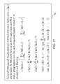
- processing unit further comprises at least one masking matrix that is a sum of an identity matrix and at least one summand masking matrix multiplied by a weight, said summand masking matrix setting certain components of a fourth orthogonal expansion of a subvector of a fourth feature vector input to said processing unit equal to zero, as said masking matrix is multiplied to said fourth orthogonal expansion, said fourth orthogonal expansion comprising components of said subvector of said fourth feature vector and a plurality of products of said components of said subvector of said fourth feature vector, wherein said estimation means also uses said at least one masking matrix in computing a representation of a probability distribution of a label of said third feature vector.
- Still another embodiment of the present invention is the first major embodiment, said processing unit further comprising conversion means for converting said representation of said probability distribution produced by said estimation means into a vector being output from said processing unit as a label of said third feature vector.
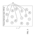
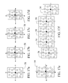
- An example subvector [2 6 14 19 23 33]′, say the third subvector, of the feature subvector n is indicated by 46 .
- the feedbacked ternary vectors which form the dynamical state of the THPAM, are usually all set equal to zero.
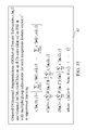
- Supervised learning means of the PU comprises adjustment means 9 for adjusting at least one GECM (general expansion correlation matrix) by receiving a GOE (general orthogonal expansion) ⁇ hacek over (x) ⁇ ⁇ (n) generated by expansion means 2 and a label r ⁇ (n) of x ⁇ (n) provided from outside the PAM and replacing said at least one GECM with a weighted sum of said at least one GECM and a product of said label r ⁇ (n) and the transpose of said GOE ⁇ hacek over (x) ⁇ ⁇ (n).
- GOE general orthogonal expansion
- a condition under which the lever is placed in the position 49 and no learning is performed is the following: If y ⁇ (n) generated by a PU's estimation means in retrieving is a bipolar vector or sufficiently close to a bipolar vector by some criterion, which indicates that the input feature subvector x ⁇ (n) is adequately learned, then the lever is placed in the position 49 and no learning is performed. This avoids “saturating” the expansion correlation matrices with one feature subvector and its label.
- feature vectors are arrays of ternary pixels.
- Other types of feature vector must be converted into arrays of ternary pixels for the methods to be described to apply.
- an image with 8-bit pixels may be converted by using a pseudo-random number generator to generate a bipolar pulse train for each pixel whose average pulse rate (i.e., the rate of +1 pulse) is proportional to 8-bit light intensity of the pixel.
- Another way to convert an image with 8-bit pixels is to replace an 8-bit pixel with 3 bipolar 2-bit pixels placed at the same location in considering rotation, translation and scaling. After conversion, at any instant of time, the feature vector is an array of ternary pixels.
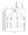
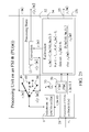
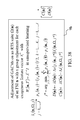
- FIG. 23 How a GOE (general orthogonal expansion) ⁇ hacek over (x) ⁇ t (n, ⁇ ) on an RTS suite ⁇ (n), is generated is shown in FIG. 23 .
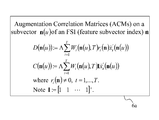
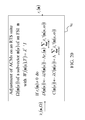
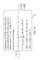
- the adjustment is performed by replacing D(n(u)) with a weighted sum of D(n(u)) and r ⁇ (n) ⁇ w ⁇ (n) ⁇ hacek over (x) ⁇ ⁇ ′(n(u,w)) and replacing C(n(u)) with a weighted sum of C(n(u)) and I ⁇ w ⁇ (n) ⁇ hacek over (x) ⁇ ⁇ ′(n(u,w)).
Abstract
A cortex-like learning machine, called a probabilistic associative memory (PAM), is disclosed for recognizing spatial and temporal patterns. A PAM is usually a multilayer or recurrent network of processing units (PUs). Each PU expands subvectors of a feature vector input to the PU into orthogonal vectors, and generates a probability distribution of the label of said feature vector, using expansion correlation matrices, which can be adjusted in supervised or unsupervised learning by a Hebbian-type rule. The PU also converts the probability distribution into a ternary vector to be included in feature subvectors that are input to PUs in the same or other layers. A masking matrix in each PU eliminates effect of corrupted components in query feature subvectors and enables maximal generalization by said PU and thereby that by the PAM. PAMs with proper learning can recognize rotated, translated and scaled patterns and are functional models of the cortex.
Description
This application claims the benefit of provisional patent application Ser. No. 61/128,499, filed 2008 May 22 by the present inventor.
In the terminology of pattern recognition, neural networks and machines learning, a feature vector is a transformation of a measurement vector, whose components are measurements or sensor outputs. This invention is mainly concerned with processing feature vectors and sequences of feature vectors for detecting and recognizing spatial and temporal causes (e.g., objects in images/video, words in speech, and characters in handwriting). This is what pattern recognition, neural networks and machines learning are essentially about. It is also a typical problem in the fields of computer vision, signal processing, system control, telecommunication, and data mining. Example applications that can be formulated as such a problem are handwritten character classification, face recognition, fingerprint identification, DNA sequence identification, speech recognition, machine fault detection, baggage/container examination, video monitoring, text/speech understanding, automatic target recognition, medical diagnosis, prosthesis control, robotic arm control, and vehicle navigation.
A good introduction to the prior art in pattern classification, neural networks and machine learning can be found in Simon Haykin, Neural Networks and Learning Machines, Third Edition, Pearson Education, New Jersey, 2009; Christopher M. Bishop, Pattern Recognition and Machine Learning, Springer Science, New York, 2006; Neural Networks for Pattern Recognition, Oxford University Press, New York, 1995; B. D. Ripley, Pattern Recognition and Neural Networks, Cambridge University Press, New York, 1996; S. Theodoridis and K. Koutroumbas, Pattern Recognition, Second Edition, Academic Press, New York, 2003; Anil K. Jain, Robert P. W. Duin and Jianchang Mao, “Statistical Pattern Recognition: A Review,” in IEEE Transactions on Pattern Analysis and Machine Intelligence, Vol. 22, No. 1, January 2000; R. O. Duda, P. E. Hart, and D. G. Stork, Pattern Classification, second edition, John Wiley & Sons, New York, 2001; and Bernhard Scholkopf and Alexander J. Smota, Learning with Kernels, The MIT Press, Cambridge, Mass., 2002.
Commonly used pattern classifiers include template matching, nearest mean classifiers, subspace methods, 1-nearest neighbor rule, k-nearest neighbor rule, Bayes plug-in, logistic classifiers, Parzen classifiers, Fisher linear discriminants, binary decision trees, multilayer perceptrons, radial basis networks, and support vector machines. They each are suitable for some classification problems. However, in general, they all suffer from some of such shortcomings as difficult training/design, much computation/memory requirement, ad hoc character of the penalty function, or poor generalization/performance. For example, the relatively more powerful multilayer perceptrons and support vector machines are difficult to train, especially if the dimensionality of the feature vectors is large. After training, if new training data is to be learned, the trained multilayer perceptron or support vector machine is usually discarded and new one is trained over again. Its decision boundaries are determined by exemplary patterns from all classes. Furthermore, if there are a great many classes or if there are no or not enough exemplary patterns for some “confuser classes” such as for target and face recognition, training an MLP or SVM either is impractical or incurs a high misclassification rate. Camouflaged targets or occluded faces not included in the training data are known to also cause high misclassification rates.
A pattern classification approach, that is relatively seldom mentioned in the pattern recognition literature, is the correlation matrix memories, or CMMs, which have been studied essentially in the neural networks community (T. Kohonen, Self-Organization and Associative Memory, second edition, Springer-Verlag, 1988; R. Hecht-Nielsen, Neurocomputing, Addison-Wesley, 1990; Branko Soucek and The Iris Group, Fuzzy, Holographic, and Parallel Intelligence—The Sixth-Generation Breakthrough, edited, John Wiley and Sons, 1992; James A. Anderson, An Introduction to Neural Networks, The MIT Press, 1995; S. Y. Kung, Digital Neural Networks, Pearson Education POD, 1997; D. J. Willshaw, P. P. Buneman and H. C. Longet-Higgins, “Non-holographic associative memory,” Nature, 222, pp. 960-962, 1969; D. J. Willshaw and H. C. Longet-Higgins, “Associative memory models,” Machine Intelligence, vol. 5, edited by B. Meltzer & O. Michie, Edinburgh University Press, 1970; K. Nagano, “Association—a model of associative memory,” IEEE Transactions on Systems, Man and Cybernetics, vol. SMC-2, pp. 68-70, 1972; G. Palm, “On associative memory,” Biological Cybernetics, vol. 36, pp. 19-31, 1980; E. Gardner, “The space of interactions in neural network models,” Journal of Physics, vol. A21, pp. 257-270, 1988; S. Amari, “Characteristics of sparsely encoded associative memory,” Neural Networks, vol. 2(6), pp. 451-457, 1989; J. Buckingham and D. Willshaw, “On setting unit thresholds in an incompletely connected associative net,” Network, vol. 4, pp. 441-459, 1993; M. Turner and J. Austin, “Matching Performance of Binary Correlation Matrix Memories,” Neural Networks, 1997). The training of CMMs, which are associative memories, is easy and fast even if they have a very high dimensional input. If new training data is to be learned or if the dimensionality of a trained CMM is to be modified, the CMM is not discarded, but can be easily updated or expanded.
Two types of CMM are noteworthy. They are the holographic neural nets (John Sutherland, “Artificial neural device utilizing phase orientation in the complex number domain to encode and decode stimulus response patterns,” U.S. Pat. No. 5,214,745, May 25, 1993; John Sutherland, “Neural networks,” U.S. Pat. No. 5,515,477, May 7, 1996) and the binary CMMs in the aforementioned papers by Willshaw and Longuet-Higgins (1970), Palm (1980), Gardner (1988), S. Amari (1989), M. Turner and J. Austin (1997), and the references therein.
The main idea of holographic neural nets (HNets) is representing real numbers by phase angle orientations on a complex number plane through the use of a sigmoidal transformation such as a hyperbolic tangent function. After each component of the input stimuli and output responses is converted into a complex number whose phase angle orientation (i.e. argument) represents the component, the correlation matrix is constructed in the standard manner. A holographic neural cell comprises essentially such a correlation matrix. If the dimensionality of the stimulus is large enough, augmented if necessary, and if the phase angle orientations of the stimuli and responses are more or less statistically independent and uniformly distributed on the unit circles in the complex number plane, the “signal part” in the response to an input stimulus is hopefully much greater than the “interference part” in the response to the same input stimulus during its retrieval because of self-destruction of those stored stimuli that are out of phase with said input stimulus like the self-destruction of a random walk on the complex number plane. This idea allows more stimuli to be stored in a complex correlation matrix than does the earlier versions of the correlation matrix.
However, the holographic neural cell approach suffers from the following shortcomings. First, to avoid ambiguity at the point, (−1, 0)=−1+0i, in the complex plane, a neighborhood of (−1, 0) must be excluded in the range of the sigmoidal transformation. This prevents the mentioned uniform distribution required for good self-destruction of the interference part. Second, it is not clear how to augment the stimuli without introducing much correlations among the stimuli, which again may reduce self-destruction of the interference part. Third, the argument of a complex number on the unit circle ranges from −π to π. To pack more stimuli on it, better self-destruction of the interference part is needed, which in turn requires a higher dimensionality of the stimuli. Such a higher dimensionality means a higher dimensionality of the correlation matrix, requiring more memory space to hold the matrix.
Binary CMMs have feature vectors encoded either into unipolar binary vectors with components equal to 1 or 0 or into bipolar binary vectors with components equal to 1 or −1. Bipolar binary vectors were used in most of the earlier work on binary CMMs. Superiority of sparse unipolar binary encoding (with most of the components of encoded feature vectors being 0 and only a few being 1) to nonsparse unipolar binary encoding and bipolar binary encoding was remarked and proved in the mentioned papers by Willshaw and Longuet-Higgins (1970), Palm (1980), Gardner (1988), and S. Amari (1989). Sparsely encoded CMMs are easy to implement (J. Austin and J. Kennedy, “A hardware implementation of a binary neural network,” MicroNeuro, IEEE Computer Press, 1994), and have found many applications. Nevertheless, sparsely encoded CMMs have quite a few shortcomings: (a) A large sparse correlation matrix has very low “information density” and takes much memory space. (b) A multistage sparsely encoded CMMs is often necessary. (c) There is no systematic way to determine the dimensionality of the sparse unipolar binary vectors to represent the feature vectors. (d) There is no systematic way to determine the number of stages or the number of neurons in each stage in a multistage sparsely encoded CMM. (e) There is no systematic way to determine whether a sparsely encoded CMM has a minimum misclassification probability for the given CMM architecture. (f) The mapping from the feature vectors to their sparse binary vectors representations must be stored in some memory space, further reducing the overall memory density of the CMM.
Judging from the foregoing shortcomings of the commonly used pattern classifiers, the holographic neural nets, and the sparsely encoded CMMs, there remains a need for alternatives to existing pattern classifiers in the prior art for recognizing patterns.
In this invention disclosure, a cortex-like learning machine, called a probabilistic associative memory (PAM), is disclosed that processes feature vectors or sequence of feature vectors, each feature vector being a ternary feature vector.
A PAM is a network of processing units (PUs). It can be viewed as a new neural network paradigm or a new type of learning machine. Each PU generates a representation of a subjective probability distribution of the label of a feature subvector or a sequence of feature subvectors that are received by the PU. Some PUs convert such representations into ternary vectors, which are included in feature subvectors input to other PUs. Weights in a PU learn an input feature subvector with or without supervision by a Hebb rule of learning. Some advantages of PAMs are the following:
-
- 1. As opposed to most of commonly used pattern recognizers, a PAM generalizes not by only a single holistic similarity criterion for the entire input exogenous feature vector, which noise, erasure, distortion and occlusion can easily defeat, but by a large number of similarity criteria for feature subvectors input to a large number of PUs (processing units) in different layers. These criteria contribute individually and collectively to generalization for single and multiple causes. Example 1: smiling; putting on a hat; growing or shaving beard; or wearing a wig can upset a single similarity criterion used for recognizing a face in a mug-shot photograph. However, a face can be recognized by each of a large number of feature subvectors of the face. If one of them is recognized to belong to a certain face, the face is recognized. Example 2: a typical kitchen contains a refrigerator, a counter top, sinks, faucets, stoves, fruit and vegetable on a table, etc. The kitchen is still a kitchen if a couple of items, say the stoves and the table with fruit and vegetable, are removed.
- 2. Masking matrices in a PU eliminate effects of corrupted ternary components of the feature subvector input to the PU, and thereby enable maximal generalization capability of the PU, and in turn that of the PAM.
- 3. PAMs are neural networks, but are no more blackboxes with “fully connected” layers much criticized by opponents of such neural networks as multilayer perceptrons (MLPs) and recurrent MLPs, whose weights are iteratively determined through minimizing an error criterion and have no interpretation in the context of their applications. In a PU of a PAM, weights are correlations between orthogonal expansions of subvectors of the PU's input feature subvectors and the labels of these feature subvectors. Each PU has a receptive region in the exogenous feature vector input to the PAM and classifies any cause within the receptive region. Such interpretations can be used to help select the architecture (i.e., layers, PUs, connections, feedback structures, etc.) of a PAM for the application.
- 4. The weights in each PU of a PAM learn by a Hebb rule and thus the PAM has a “photographic memory.” No iterative optimization such as that involved in local-search training methods using backpropagation or backpropagation through time is needed for learning. This allows easy learning of a large number of large exogenous feature vectors in reasonable time as well as easy online adaptive learning.
- 5. A PU can learn with or without supervision. This allows a PAM to (1) perform unsupervised deep learning in lower layers and supervised learning in higher layers; (2) perform supervised learning when a label is provided from outside the PAM and unsupervised learning when not; and (3) perform autonomous learning.
- 6. A PAM may have some capability of recognizing rotated, translated and scaled patterns. Moreover, easy learning and retrieving by a PAM allow it to learn translated, rotated and scaled versions of an input image with ease.
- 7. PUs generate representations of probability distributions of the labels of their input feature subvectors. Such representations of probability distributions of a common label can be combined into a single representation of probability distributions of the common label.
- 8. PAMs with hierarchical and feedback structures can detect and recognize multiple and hierarchical causes in a spatial or temporal exogenous feature vector.
- 9. The weight matrices (e.g., expansion correlation matrices) in different PUs can be added to combine the learned knowledge at virtually no additional cost.
- 10. The architecture of a PAM can be adjusted without discarding learned knowledge in the PAM. This allows enlargement of the feature subvectors, increase of the number of layers, and even increase of feedback connections.
- 11. Only a small number of algorithmic steps of parallel computing are needed for retrieval, which are suitable for massive parallelization at the bit level and by VLSI implememtation.
The present invention is embodied in systems, learning machines or methods. In this Section: SUMMARY, embodiments in a system are stated. Replacing the term, “system”, in these statements of system embodiments with the term, “learning machine”, yields statements of embodiments in a learning machine. It is understood that these statements of embodiments in a learning machine are incorporated in this Section, although they are not explicitly provided.
An objective of the present invention is to provide a system that learns to recognize spatial or temporal patterns or causes.
Another objective of the present invention is to provide a system that can learn and recognize partially erased, smeared, noise-corrupted, covered, distorted, or altered patterns.
Still another objective of the present invention is to provide a system that can perform supervised or unsupervised learning or both.
Still another objective of the present invention is to provide a system whose architecture can be adjusted without discarding already learned knowledge.
Still another objective of the present invention is to provide a system that produces representations of probability distributions of labels of feature vectors and subvectors.
Still another objective of the present invention is to provide a system with a hierarchical structure for recognizing hierarchical causes (or patterns) at different levels such as line segments in a letter, or ears, nose, mouth and eyes on a face, or apples and oranges in baskets on a table.
Still another objective of the present invention is to provide a system with feedback structures for processing sequences of related exogenous feature vectors such as those obtained from examining one single image for a plurality of consecutive time points, images of an object from different angles, consecutive frames in a video or movie, and handwritten letters in a word, words in a sentence, and sentences in a paragraph.
Still another objective of the present invention is to provide a system that can recognize rotated, translated and/or scaled versions of images that have been learned by the system.
Still another objective of the present invention is to provide a system that learns autonomously.
The foregoing objectives, as well as other objectives of the present invention that will become apparent from the discussion below, are achieved by the present invention with the following preferred embodiments.
A first major embodiment of the present invention disclosed herein is a system (or learning machine) for processing feature vectors. Such feature vectors that are input to the system are also called exogenous feature vectors to distinguish them from feature vectors that contain components generated internally by said system. The first major embodiment comprises at least one processing unit that comprises
-
- expansion means for generating, in response to a first feature vector input to said processing unit, a first orthogonal expansion of a subvector of said first feature vector, said first orthogonal expansion comprising components of said subvector of said first feature vector and a plurality of products of said components of said subvector of said first feature vector;
- at least one first expansion correlation matrix that is a weighted sum of outer products, each being an outer product of a linear combination (or weighted sum) of a vector with components all equal to 1 and a label of a second feature vector input to said processing unit and a second orthogonal expansion of a subvector of said second feature vector, said second orthogonal expansion comprising components of said subvector of said second feature vector and a plurality of products of said components of said subvector of said second feature vector; and
- estimation means for using at least said at least one first expansion correlation matrix and at least one third orthogonal expansion of a subvector of a third feature vector input to said processing unit, said third orthogonal expansion being generated by said expansion means in response to said third feature vector, to compute a representation of a probability distribution of a label of said third feature vector.
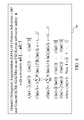
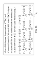
Note that an orthogonal expansion {hacek over (v)} of a vector v with m components is displayed in (2). A way to generate {hacek over (v)} is to start with {hacek over (v)}(1)=[1 v1]′ and then keep using the recursive formula (I) until {hacek over (v)}={hacek over (v)}(1, . . . , m) is obtained.
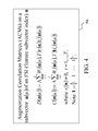
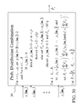
Note that said second expansion correlation matrix is a weighted sum of outer products, each being an outer product (c1I+c2rt(n)){hacek over (x)}t′(n(u)) of a linear combination (or weighted sum) c1I+c2rt(n) of a vector I=[1 . . . 1]′ with all components equal to 1 and a label rt(n) of a feature vector xt(n) input to said processing unit and an orthogonal expansion {hacek over (x)}t(n(u)) of the subvector xt(n(u)) of the feature vector xt(n), where t=1, . . . , T for some positive integer T, and c1 and c2 are real-valued weights. Expansion correlation matrices with specific values of c1 and c2 are shown in FIG. 4 and (3), (4), (5) and (6). Note that pτ(n) is also a representation of the probability distribution.
Note that a label of a feature vector input to a processing unit is defined as follows: A PU in a PAM has a “receptive field” in the exogenous feature vector and a “receptive field” in the measurement vector. These two receptive fields can be found by tracing the feedforward connections in the PAM backforward from a feature vector input to the PU (or the feature subvector index of the PU) to an exogenous feature vector (or the input terminals) of the PAM, and then tracing the transformation, that maps the measurement vector into the exogenous feature vector, backward from the exogenous feature vector to the measurement vector. The components of the measurement vector that can be reached by this backward tracing from a PU to the exogenous feature vector and then to the measurement vector are called the “receptive field” of the PU in the measurement vector. The components of the exogenous feature vector that can be reached by this backward tracing from a PU to the exogenous feature vector are called the “receptive field” of the PU in the exogenous feature vector. The label of a feature vector input to a PU is the label of the corresponding components of measurement vector in the receptive field of the PU in the measurement vector. The label of the corresponding components of the exogenous feature vector in the receptive field of the PU in the exogenous feature vector is also this label.
Note that the weights in said weighted sum of outer products are ΛWt(n(u), T), t=1, . . . , T. If the matrix W, (n(u), T) is a diagonal matrix with equal entries, then the weights in the weighted sum of outer products are actually scalar weights. Two examples are Wt(n(u), T)=λT-tI and Wt(n(u), T)=I/√{square root over (T)}. Therefore, the weights in the weighted sum of outer products in the first major embodiment are either matrix weights or scalar weights.
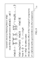
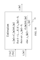
Note that an estimation means for generating a representation yτ(n) of a probability distribution pτ(n) of the label rτ(n) of xτ(n) is shown in FIG. 10 and described in Subsection 5.3, “Representations of Probability Distributions”.
Another embodiment of the present invention is the first major embodiment, wherein said processing unit further comprises at least one masking matrix that is a sum of an identity matrix and at least one summand masking matrix multiplied by a weight, said summand masking matrix setting certain components of a fourth orthogonal expansion of a subvector of a fourth feature vector input to said processing unit equal to zero, as said masking matrix is multiplied to said fourth orthogonal expansion, said fourth orthogonal expansion comprising components of said subvector of said fourth feature vector and a plurality of products of said components of said subvector of said fourth feature vector, wherein said estimation means also uses said at least one masking matrix in computing a representation of a probability distribution of a label of said third feature vector.
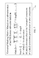
Note that a masking matrix M(n(u)) is displayed in FIG. 7 and (26). The masking matrix M(n(u)) is a sum of an identity matrx I and
Because diag({hacek over (I)}(i1 −, i2 −, . . . , ij −)) appears in a
Another embodiment of the present invention are the first major embodiment of the present invention, wherein c1=0 and c2=1 in the linear combination or weighted sum c1I+c2rt(n). In this embodiment the second expansion correlation matrix is D(n(u)) displayed in FIG. 4 and (3).
Another embodiment of the present invention is the first major embodiment of the present invention, wherein c1=1 and c2=0 in the linear combination c1I+c2rt(n). In this embodiment the second expansion correlation matrix is C(n(u)) displayed in FIG. 4 and (4).
Another embodiment of the present invention is the first major embodiment of the present invention, wherein c1=1 and c2=1 in the linear combination c1I+c2rt(n). In this embodiment the second expansion correlation matrix is C(n(u)) displayed in (5).
Another embodiment of the present invention is the first major embodiment of the present invention, wherein c1=1 and c2=−1 in the linear combination c1I+c2rt(n). In this embodiment the second expansion correlation matrix is B(n(u)) displayed in (6).
Another embodiment of the present invention is the first major embodiment wherein weights in said weighted sum of outer products are equal.
Another embodiment of the present invention is the first major embodiment, wherein at least one expansion correlation matrix is an expansion correlation matrix on a rotation/translation/scaling (RTS) suite of a subvector of a feature subvector index.
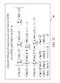
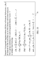
Note that such expansion correlation matrices are shown in FIGS. 19 and (40)-(43), where the rotation/translation/scaling suite is denoted by Ω(n). These expansion correlation matrices help the above embodiment recognize rotated, translated and scaled causes or objects.
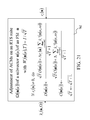
Still another embodiment of the present invention is the first major embodiment, said processing unit further comprising supervised learning means for adjusting, in response to a fifth feature vector input to said processing unit, said at least one first expansion correlation matrix by using at least an outer product of a linear combination of a vector with components all equal to 1 and a label of said fifth feature vector input to said processing unit and a fifth orthogonal expansion of a subvector of said fifth feature vector, said fifth orthogonal expansion comprising components of said subvector of said fifth feature vector and a plurality of products of said components of said subvector of said fifth feature vector, wherein said label of said fifth feature vector is provided from outside said learning machine.
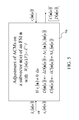
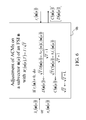
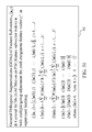
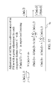
Note that supervised learning is discussed in Subsection 5.6, “Processing Units and Supervised/Unsupervised Learning”. Examples of adjusting expansion correlation matrices, D(n(u)) and C(n(u)), in supervised learning by using outer products, rt(n){hacek over (x)}t′(n(u)) and I{hacek over (x)}t′(n(u)), respectively, are shown in FIG. 5 and FIG. 6 , where the label rt(n) of the feature vector xt(n) input to said processing unit is provided from outside the system or learning machine.
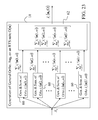
Still another embodiment of the present invention is the first major embodiment, said processing unit further comprising conversion means for converting said representation of said probability distribution produced by said estimation means into a vector being output from said processing unit as a label of said third feature vector.
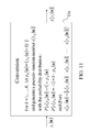
Note that conversion of a representation of a probability distribution is discussed in Subsection 5.5. Two conversion means are described in the Section and are shown in FIG. 11 and FIG. 12 .
Still another embodiment of the present invention, called embodiment 1, is the first major embodiment, said processing unit further comprising a pseudo-random vector generating means for generating a pseudo-random vector in accordance with said probability distribution produced by said estimation means, said pseudo-random vector being output from said processing unit as a label of said third feature vector.
Note that the pseudo-random vector generating means is shown in FIG. 12 and is the second conversion method described in Subsection 5.5.
Still another embodiment of the present invention is embodiment 1, said processing unit further comprising unsupervised learning means for adjusting, in response to a sixth feature vector input to said processing unit, said at least one first expansion correlation matrix by using at least one outer product of a linear combination of a vector with components all equal to 1 and a label of said sixth feature vector and a sixth orthogonal expansion of a subvector of said sixth feature vector, said sixth orthogonal expansion comprising components of said subvector of said sixth feature vector and a plurality of products of said components of said subvector of said sixth feature vector, wherein said label of said sixth feature vector is a pseudo-random vector generated by said pseudo-random vector generating means as a label of said sixth feature vector.
Note that unsupervised learning is discussed in Subsection 5.6, “Processing Units and Supervised/Unsupervised Learning”. Examples of adjusting expansion correlation matrices, D(n(u)) and C(n(u)), by using outer products, rt(n){hacek over (x)}t′(n(u)) and I{hacek over (x)}t′(n(u)), respectively, are shown in FIG. 5 and FIG. 6 , where the label rt(n) of said sixth feature vector xt(n) is said pseudo-random vector generated by said pseudo-random vector generating means as a label of said sixth feature vector.
Still another embodiment of the present invention is embodiment 1, wherein a plurality of components of a pseudo-random vector that is output from a processing unit are components of a feature vector that is input to another processing unit.
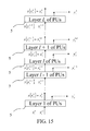
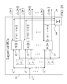
Note that in this embodiment, there are at least 2 processing units. A plurality of components of a pseudo-random vector output from one of the processing units are components of a feature vector input to another processing unit. Said at least 2 processing units form a network of processing units, which may be a multilayer network of processing units. A multilayer network of processing units is shown in FIG. 15 .
Still another embodiment of the present invention is embodiment 1, wherein a plurality of said at least one processing unit form a network with a plurality of ordered layers of said processing units; each exogenous feature vector is input to layer 1 of said network, which is the lowest-ordered layer of said network; and components of a feature vector input to a processing unit in layer l of said network, where l>1, are components of at least one label that is output from at least one processing unit in layer l-1 of said network.
Note that a multilayer network of processing units is shown in FIG. 15 .
Still another embodiment of the present invention is embodiment 1 for processing exogenous feature vectors in sequences of exogenous feature vectors, wherein a plurality of components of a pseudo-random vector that is output from a processing unit in processing a certain exogenous feature vector in a sequence of exogenous feature vectors are included as components, after a time delay, in a feature vector that is input to a processing unit in processing an exogenous feature vector subsequent to said certain exogenous feature vector in said sequence.
Note that in this embodiment, a plurality of components of a pseudo-random vector output from a processing unit are, after a time delay, components of a feature vector input to another processing unit. Because of the time delay, said at least 2 processing units can form a network of processing units with “feedback connections”, which is a dynamical system by itself.
Still another embodiment of the present invention is embodiment 1 for processing exogenous feature vectors in sequences of exogenous feature vectors, wherein at least one component of a label that is output from a processing unit in layer j in processing a certain exogenous feature vector in a sequence is included as a component, after a time delay, in a feature vector that is input to a processing unit in layer k, where k≦j, in processing an exogenous feature vector subsequent to said certain exogenous feature vector in said sequence. A multilayer network of processing units with feedbacks is shown in FIG. 16 .
A second major embodiment is a method for processing feature vectors, said method comprising:
-
- an expanding step of expanding a subvector of a first feature vector into a first orthogonal expansion that comprises components of said subvector of said first feature vector and a plurality of products of said components of said subvector of said first feature vector, and
- an estimating step of using
- 1. at least one orthogonal expansion of a subvector of said first feature vector produced by said expanding step; and
- 2. at least one expansion correlation matrix that is a weighted sum of outer products, each being an outer product of a weighted sum of a vector with components all equal to 1 and a label of a second feature vector and a second orthogonal expansion of a subvector of said second feature vector, said second orthogonal expansion comprising components of said subvector of said second feature vector and a plurality of products of said components of said subvector of said second feature vector;
to compute a representation of a probability distribution of a label of said first feature vector.
Note that all the terms used in the above second major embodiment are those used in the first major embodiment, which are briefly described for the first major embodiment. Note also that the terms used in all the embodiments below are those used in the embodiments above following the first major embodiment.
Another embodiment of the present invention is the second major embodiment, wherein said estimating step also uses at least one masking matrix that is a sum of an identity matrix and at least one summand masking matrix multiplied by a weight, said summand masking matrix setting certain components of a third orthogonal expansion of a subvector of a third feature vector equal to zero, as said masking matrix is multiplied to said third orthogonal expansion, to compute a representation of a probability distribution of a label of said first feature vector, said third orthgonal expansion comprising components of said subvector of said third feature vector and a plurality of products of said components of said subvector of said third feature vector.
Another embodiment of the present invention is the second major embodiment, wherein said weighted sum of a vector with components all equal to 1 and a label of a second feature vector is said label of said second feature vector.
Another embodiment of the present invention is the second major embodiment, wherein said weighted sum of a vector with components all equal to 1 and a label of a second feature vector is said vector with components all equal to 1.
Another embodiment of the present invention is the second major embodiment, wherein said weighted sum of a vector with components all equal to 1 and a label of a second feature vector is a sum of said vector with components all equal to 1 and said label of said second feature vector
Another embodiment of the present invention is the second major embodiment, wherein weights in said weighted sum of outer products are equal.
Another embodiment of the present invention, called embodiment 2, is the second major embodiment, further comprising a generating step of generating a pseudo-random vector in accordance with said probability distribution as a label of said first feature vector.
Another embodiment of the present invention is embodiment 2, further comprising a feedforward step of including a plurality of components of a pseudorandom vector generated by said generating step as a label of said first feature vector as components in a fourth feature vector and processing said fourth feature vector by said expanding step and said estimating step.
Another embodiment of the present invention is embodiment 2, further comprising a feedback step of including, after a time delay, a plurality of components of a pseudorandom vector generated by said generating step as a label of said first feature vector as components in a fifth feature vector and processing said fifth feature vector by said expanding step and said estimating step.
Another embodiment of the present invention is embodiment 2, further comprising an unsupervised learning step of adjusting said expansion correlation matrix by using at least one outer product of a weighted sum of a vector with components all equal to 1 and a label of a sixth feature vector and an orthogonal expansion of a subvector of said sixth feature vector produced by said expanding step, wherein said label of said sixth feature vector is a pseudo-random vector generated by said generating step as a label of said sixth feature vector.
Another embodiment of the present invention is embodiment 2, further comprising a supervised learning step of adjusting said expansion correlation matrix by using at least an outer product of a weighted sum of a vector with components all equal to 1 and a label of a seventh feature vector and an orthogonal expansion of a subvector of said seventh vector produced by said expanding step, wherein said label of said seventh feature vector is provided.
Embodiments of the invention disclosed herein, which are called probabilistic associative memories (PAMs), comprise at least one processing unit (PU). Component parts of a PU are first shown in the drawings described below. Drawings are then given to show how these component parts are used to construct some embodiments of the present invention. Embodiments of the present invention that can recognize rotated, translated and scaled causes (e.g., objects) and their component parts are also shown in drawings.
In the present invention disclosure, the prime denotes matrix transposition, and a vector is regarded as a subvector of the vector itself, as usual.
{hacek over (v)}(1, . . . ,j+1)=[{hacek over (v)}′(1, . . . ,j)v j+1 {hacek over (v)}′(1, . . . ,j)]′,
evaluates {hacek over (v)}(1, . . . , j) for j=2, . . . , k−1, yielding {hacek over (v)}={hacek over (v)}(1, . . . , k).
A PAM usually has a plurality of ordered layers, and a layer usually has a plurality of PUs (processing units). A vector input to layer l is called a feature vector and denoted by xt l-1=[xt1 l-1 xt2 l-1 . . . xtM l-1]′, t is used to distinguish feature vectors that are input at different times (or with different numberings). A vector that is input to a PU (processing unit) in layer l is a subvector of a feature vector xt l-1. The subvector index of said subvector of the feature vector xt l-1 is called a feature subvector index (FSI). A feature subvector index (FSI) is denoted by a lower-case boldface letter. A symbol to denote a typical FSI is n and the subvector xt l-1 (n) is called the feature subvector on the FSI n.
instead. Here C(n(u)) is a row vector, and the ECM [C′(n(u)) (n(u))]′ has R+1 rows.
diag({hacek over (I)}(i1 −, i2 −, . . . , ij −)) appears in a summand 2−8j2jdiag({hacek over (I)}(i1 −, i2 −, . . . , ij −)) in (26) for the masking matrix M(n(u)), the matrix diag({hacek over (I)}(i1 −, i2 −, . . . , ij −)) is called a summand masking matrix in M(n(u)). A summand 2−8j2jdiag({hacek over (I)}(i1 −, i2 −, . . . , ij −)) in (26) is a summand masking matrix diag({hacek over (I)}(i1 −, i2 −, . . . , ij −)) multiplied by a weight 2−8j2j. When M(n(u)) is multiplied to an orthogonal expansion {hacek over (x)}τ(n(u)) of a subvector xτ(n(u)) of xτ, each diag({hacek over (I)}(i1 −, i2 −, . . . , ij −)) in FIG. 7 or (26) is multiplied to {hacek over (x)}τ(n(u)) to get diag({hacek over (I)}(i1 −, i2 −, . . . , ij −)) xτ(n(u)), in which the components of {hacek over (x)}τ(n(u)) that involve the i 1-th, i2-th, . . . , and ij-th components of xτ(n(u)) are set equal to 0. A masking matrix M(n(u)) is used to set automatically selected components of a subvector xτ(n(u)) of a feature subvector xτ(n) equal to 0 in order to retrieve the label of a feature subvector stored in ECMs that shares the largest number of components with xτ(n(u)). Note that 2−8 is an example weight factor selected to differentiate between different levels of maskings to effect the automatic selection. The weight should be selected to suit the application. Note that as usual, I denotes an identity matrix, and I=diag I.
The output x{yτ(n)} that conversion means generates is an R-dimensional vector with components x{yτk(n)}, k=1, . . . , R. x{yτ(n)} is a point estimate of rτ(n).
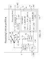
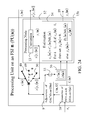
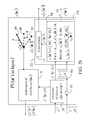
If a label rτ(n)≠0 of xτ(n) from outside the PU is available for learning, and learning xτ(n) and rτ(n) is wanted, supervised learning is performed by the PU. In supervised learning, the label rτ(n)≠0 is received through a lever represented by a thick solid line with a solid dot in the position 48 by an adjustment means 9, which receives also {hacek over (x)}τ(n) from the expansion means 2 and uses a method of adjusting ECMs such as those depicted in FIG. 5 and FIG. 6 and assembles the resultant ECMs C(n(u)) and D(n(u)), u=1, . . . , U, into general ECMs
C(n)=[C(n(1))C(n(2)) . . . C(n(U))]
D(n)=[D(n(1))D(n(2)) . . . D(n(U))]
These C(n) and D(n) are then stored, after a one-numbering delay (or a unit-time delay) 33, in thestorage 56, from which they are sent to the estimation means 54. The one-numbering delay is usually a time delay that is long enough for the estimation means to finish using current C(n) and D(n) in generating and outputting yτ(n), but short enough for getting the next C(n) and D(n) generated by the adjustment means available for the estimation means to use for processing the next orthogonal expansion or general orthogonal expansion from the expansion means.
C(n)=[C(n(1))C(n(2)) . . . C(n(U))]
D(n)=[D(n(1))D(n(2)) . . . D(n(U))]
These C(n) and D(n) are then stored, after a one-numbering delay (or a unit-time delay) 33, in the
Supervised learning means is described as follows: If a class label rτ(n)≠0 of xτ(n) from outside PU(n) is available and learning xτ(n) and rτ(n) is wanted, supervised learning means of the PU for adjusting at least one GECM (general expansion correlation matrix) performs supervised learning by receiving a GOE (general orthogonal expansion) {hacek over (x)}τ(n) generated by expansion means 2 and a label rτ(n)≠0 of xτ(n) provided from outside the PAM, using adjustment means 9 to adjust each ECM block in GECMs.
If a label rτ(n) of xτ(n) from outside the PU is unavailable but learning xτ(n) is wanted, unsupervised learning is performed by the PU. In this case, the lever (shown in position 48 in FIG. 13 ) should be in the position 50. The feature subvector xτ(n) is first processed by the expansion means 2, estimation means 54, conversion means 13 as in performing retrieval described above. The resultant ternary vector x{yτ(n)} is received, through the lever in position 50, and used by the adjustment means 9 as the label rτ(n) of xτ(n). The adjustment means 9 receives {hacek over (x)}τ(n) also and uses a method of adjusting ECMs such as those depicted in FIG. 5 and FIG. 6 and assembles the resultant ECMs, C(n(u)) and D(n(u)), u=1, . . . , U, into general ECMs
C(n)=[C(n(1))C(n(2)) . . . C(n(U))]
D(n)=[D(n(1))D(n(2)) . . . D(n(U))]
These C(n) and D(n) are then stored, after a one-numbering delay (or a unit-time delay) 33, in thestorage 56, from which they are sent to the estimation means 54.
C(n)=[C(n(1))C(n(2)) . . . C(n(U))]
D(n)=[D(n(1))D(n(2)) . . . D(n(U))]
These C(n) and D(n) are then stored, after a one-numbering delay (or a unit-time delay) 33, in the
Unsupervised learning means is described as follows: If a label rτ(n) of xτ(n) from outside PU(n) is unavailable but learning xτ(n) is wanted, unsupervised learning means of the PU for adjusting at least one GECM (general expansion correlation matrix) performs unsupervised learning by receiving a GOE (general orthogonal expansion) {hacek over (x)}τ(n) generated by expansion means 2 and a ternary vector x{yτ(n)} generated by the conversion means 13 and using adjustment means 9 to adjust each ECM block in GECMs.
If no learning is to be performed by PU(n), the lever represented by a thick solid line with a solid dot is placed in the position 49, through which 0 is sent as the label rτ(n) of xτ(n) to the adjustment means 9, which then keeps C(n) and D(n) unchanged or stores the same C(n) and D(n) in the storage 56 after a one-numbering delay (or a unit-time delay).
For instance, in processing a sequence {xt ex, t=1, 2, . . . } of exogenous feature vectors input to the PAM, the output x{yτ-1 3} of layer 3 of PUs in processing xτ-1 ex, which has been held in a delay device, is included in the feature vector xτ 2 input to the same layer,
x τ 2 =[x′{y τ-1 4 }x′{y τ 2 }x′{y τ-1 3}]′
through thefeedback path 373 in processing xτ ex, which is subsequent to xτ-1 ex in the same sequence {xt ex, t=1, 2, . . . }. x{yτ-1 3} is also included in the feature vector input to layer 2 of PUs,
x τ 1 =[x′{y τ-1 3 }x′{y τ 1 }x′{y τ-1 2}]′
through thefeedback path 353, in processing xτ ex, which is subsequent to xτ-1 ex in the same sequence {xt ex, t=1, 2, . . . }.
x τ 2 =[x′{y τ-1 4 }x′{y τ 2 }x′{y τ-1 3}]′
through the
x τ 1 =[x′{y τ-1 3 }x′{y τ 1 }x′{y τ-1 2}]′
through the
Before a new sequence of exogenous feature vectors is started to be processed, the feedbacked ternary vectors, which form the dynamical state of the THPAM, are usually all set equal to zero.
Note that the exogenous feature vector xτ ex input to the PAM is part of the feature vector xτ 0 that is input to layer 1 of the PAM.
on the RTS suite Ω(n(u)) of n(u).
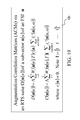
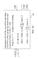
If a label rτ(n)≠0 of xτ(n) from outside the PU is available for learning, and learning xτ(n) and rτ(n) is wanted, supervised learning is performed by the PU. In supervised learning, the label rτ(n)≠0 is received through a lever represented by a thick solid line with a solid dot in the position 48 by an adjustment means 9, which receives also {hacek over (x)}(n,Ω) and uses a method of adjusting expansion correlation matrices (ECMs) on an RTS suite Ω(n(u)) such as those depicted in FIG. 20 and FIG. 21 and assembles the resultant ECMs C(n(u)) and D(n(u)) on Ω(n(u)), u=1, . . . , U, into general ECMs on the RTS suite Ω(n)={Ω(n(1)), Ω(n(2)), . . . , Ω(n(U))},
C(n)=[C(n(1))C(n(2)) . . . C(n(U))]
D(n)=[D(n(1))D(n(2)) . . . D(n(U))]
These C(n) and D(n) are then stored, after a one-numbering delay (or a unit-time delay) 33, in thestorage 56, from which they are sent to the estimation means 54.
C(n)=[C(n(1))C(n(2)) . . . C(n(U))]
D(n)=[D(n(1))D(n(2)) . . . D(n(U))]
These C(n) and D(n) are then stored, after a one-numbering delay (or a unit-time delay) 33, in the
Supervised learning means is described as follows: If a label rτ(n)≠0 of xτ(n) from outside PU(n) is available and learning xτ(n) and rτ(n) is wanted, supervised learning means of the PU for adjusting GECMs (general expansion correlation matrices) on Ω(n) performs supervised learning by receiving a GOE (general orthogonal expansion) {hacek over (x)}τ(n) generated by expansion means 2 and a label rτ(n)≠0 of xτ(n), provided from outside the PAM, and using adjustment means 9 to adjust each ECM block in GECMs on Ω(n).
If a label rτ(n) of xτ(n) from outside the PU is unavailable but learning xτ(n) is wanted, unsupervised learning is performed by the PU. In this case, the lever (shown in position 48 in FIG. 13 ) should be in the position 50. The feature subvector xτ(n) is first processed by the expansion means 2, estimation means 54, conversion means 13 as in performing retrieval described above. The resultant ternary vector x{yτ(n)} is received, through the lever in position 50, and used by the adjustment means 9 as the label rτ(n) of xτ(n). The adjustment means 9 receives {hacek over (x)}τ(n,Ω) also and uses a method of adjusting ECMs such as those depicted in FIG. 20 and FIG. 21 and assembles the resultant ECMs C(n(u)) and D(n(u)) on Ω(n(u)), u=1, . . . , U, into general ECMs on Ω(n),
C(n)=[C(n(1))C(n(2)) . . . C(n(U))]
D(n)=[D(n(1))D(n(2)) . . . D(n(U))]
These C(n) and D(n) on Ω(n) are then stored, after a one-numbering delay (or a unit-time delay) 33, in thestorage 56, from which they are sent to the estimation means 54.
C(n)=[C(n(1))C(n(2)) . . . C(n(U))]
D(n)=[D(n(1))D(n(2)) . . . D(n(U))]
These C(n) and D(n) on Ω(n) are then stored, after a one-numbering delay (or a unit-time delay) 33, in the
Unsupervised learning means is described as follows: If a label rτ(n) of xτ(n) from outside PU(n) is unavailable but learning xτ(n) is wanted, unsupervised learning means of the PU for adjusting GECMs (general expansion correlation matrices) on Ω(n) performs unsupervised learning by receiving a GOE (general orthogonal expansion) {hacek over (x)}τ(n,Ω) on Ω(n) generated by expansion means 18 and the ternary vector x{yτ(n)} (generated in processing xτ(n) in performing retrieval) as the label rτ(n) of xτ(n) and using adjustment means 9 to adjust each ECM block in GECMs on Ω(n).
If no learning is to be performed by PU(n), the lever represented by a thick solid line with a solid dot is placed in the position 49, through which 0 is sent as the label rτ(n) of xτ(n) to the adjustment means 9, which then keeps C(n) and D(n) unchanged or stores the same C(n) and D(n) in the storage 56 after a one-numbering delay (or a unit-time delay).
is obtained. In the first way, {hacek over (x)}t(n,j), j=1, . . . , J, have been generated with different GECMs by PUs. In the second way, all PUs in the PAM keep their GECMs unchanged for j=1, . . . , J. The first way is called multiple adjustments of GECMs, and the second a group adjustment of the same. To faciliate multiple adjustiments, we need a delay device in each PU that holds the GECMs for 1/J unit of time, before sends them to the
is a measure of variability of pt(n,j). Roughly speaking, the more variability a random variable has, the less information it contains. Therefore, the minimizer pt(n,j*) of the sum of variances is most informative, and x{yt(n,j*)} should be used as the common label of the J feature subvectors.
In the terminology of pattern recognition, a feature vector is a transformation of a measurement vector, whose components are measurements or sensor outputs, and a label of said feature vector is a label of said measurement vector. A subvector of a feature vector is called a feature subvector. A feature subvector is itself a feature vector. As a special case, the transformation is the identity transformation, and the feature vector is the measurement vector. Example measurement vector are digital pictures, frames of a video, segments of speech, handwritten characters/words. This invention is mainly concerned with processing feature vectors and sequences of related feature vectors for detecting and recognizing spatial and temporal causes or patterns.
In this invention disclosure, a cortex-like learning machine, called a probabilistic associative memory (PAM), is disclosed that processes feature vectors or sequence of feature vectors, each feature vector being a ternary feature vector. Such feature vectors input to a PAM are called exogenous feature vectors. A PAM can be viewed as a new neural network paradigm, a new type of learning machine, or a new type of pattern recognizer. A PAM is a network of processing units (PUs). In a multilayer PAM with or without feedback connections, the vector input to a layer is a feature vector, because it is a transformation of exogenous feature vectors input to the PAM, and in turn a transformation of the measurement vector. In a PAM with (delayed) feedback connections (or feedback means), called a recurrent PAM, a feature vector input to layer/comprises a vector output from layer l-1 and vectors output and feedbacked from PUs in other layers. For example, if there is a feedback connection to layer 1, then an exogenous feature vector is not an entire feature vector input to layer 1, but only a subvector of said entire feature vector.
A PU may comprise expansion means, estimation means, conversion means, adjustment means, feedback means, supervised learning means, unsupervised learning means, and/or storage means. A feature vector input to a PU is usually a subvector of a feature vector input to the layer to which said PU belongs. The subvector input to a PU is called a feature subvector to distinguish it from the feature vector input to the layer to which said PU belongs. If no confusion is likely, the vector input to a PU is still called a feature vector. A label of a feature vector (or subvector) input to a PU in a PAM is a label of the subvector of the exogenous feature vector that is transformed in the PAM into said feature vector (or subvector) input to the PU. A PU may have one or both of two functions—retrieving the label of a feature subvector from the memory (i.e., expansion correlation memories or general expansion correlation memories disclosed in this invention) and learning a feature subvector and its label that is either provided from outside the PU (in supervised learning) or generated by the PU itself (in unsupervised learning). In performing retrieval, a feature subvector input to a PU is first expanded into a general orthogonal expansion by the expansion means (to be described later on). The general orthogonal expansion is then processed by the estimation means, using the memory from the storage, into a representation of a probability distribution of the label of said feature subvector. The conversion means converts said representation into a ternary vector, which is an output of the PU. If said representation is needed for use outside the PU, it is also output from the PU.
There are three types of PU according to how they learn—supervised PUs, unsupervised PUs, and supervised/unsupervised PU. A supervised PU performs supervised learning, if a label of a feature subvector input to the PU is provided from outside the PU (or the PAM) and learning is wanted. An unsupervised PU performs unsupervised learning if a label of a feature subvector input to the PU is not provided from outside the PU but learning the feature subvector is wanted. A supervised/unsupervised PU can perform both supervised learning and unsupervised learning. Both supervised and unsupervised learning follow a Hebb rule of learning. During the process of learning, supervised or unsupervised, the PU is said to be performing learning.
A PU with a general masking matrix (to be described later on) has good generalization capability. A PU that has learned feature subvectors on a rotation/translation/scaling suite (to be described later on) has good capability for recognizing rotated, translated and scaled patterns.
In this invention disclosure, prime ′ denotes matrix transposition. Vectors whose components are 0's, 1's and −1's are called ternary vectors. Thus, the components of ternary vectors are elements of the ternary set, {−1, 0, 1}. Bipolar binary vectors are vectors whose components are elements of the binary set, {−1, 1}. Unipolar binary vectors are vectors whose components are elements of the binary set, {0, 1}. Since {−1, 1} and {0, 1} are subsets of the ternary set, bipolar and unipolar binary vectors are ternary vectors. For example, the bipolar binary vector [1 −1 1 −1]′ and the unipolar binary vector [1 0 1 0]′ are ternary vectors.
In the present invention disclosure, exogenous feature vectors input to a PAM are ternary vectors. 0's are usually used to represent unknown, unavailable, or corrupted part or parts of exogenous feature vectors. A vector whose components are the numberings (or subscripts) of the components of a feature vector that constitute a feature subvector and are ordered by the magnitudes of the numberings is called the feature subvector index of the feature subvector. For example, [v2 v4]′ is a feature subvector of the feature vector v=[v1 v2 v3 v4]′, and the feature subvector index of the feature subvector is [2 4]′. As usual, one of the subvectors of a vector is said vector itself. Labels in the present invention disclosure are also ternary vectors. 0's are usually used to represent unavailable, unknown or unused part or parts of labels. For instance, if we start out with labels with different dimensionalities (or different numbers of components) in an application, the dimensionalities of those with smaller dimensionalities can be increased by inserting 0's at the tops or bottoms as additional components so that all the labels have the same dimensionality in the application.
An orthogonal expansion and a general orthogonal expansion of a ternary vector are described in the next subsection. A general orthogonal expansion has, as its block column(s), at least one orthogonal expansion. An orthogonal expansion is a special case of a general orthogonal expansion. A sum or weighted sum of products of values of a vector-valued function evaluated at labels of feature subvectors and transposes of general orthogonal expansions of these feature subvectors (with the same feature subvector index) is called an expansion correlation matrix (on the feature subvector index). Note that if the vector-valued function of the label is one-dimensional, the feature subvector expansion correlation matrix is a vector, sometimes called a expansion correlation vector.
In the present invention disclosure, probabilities are usually subjective probabilities, and therefore variances; estimations; distributions and statements based on probabilities are usually those based on subjective probabilities, whether the word “subjective” is used or not, unless indicated otherwise.
There are many ways to convert discrete numbers into bipolar binary vectors. A standard way to convert a base-10 number into a unipolar binary number is to convert the base-10 representation into a base-2 representation. For instance, (51)10=(110011)2. A unipolar binary number can be converted into a bipolar binary vector by changing every 0 to −1. For instance, (110011)2 is converted into [1 1 −1 −1 1 1]′. An example of converting a representation of a probability distribution, which is a R-vector with real-valued components, is illustrated in FIG. 11 , wherein each component is approximated by a 3-component unipolar binary number before being converted into a bipolar binary number by changing every 0 to −1.
The Hamming distance between the standard unipolar binary representations of two integers is not “consistent” with their real value distance in the sense that a larger Hamming distance may correspond to a smaller real-value distance. For instance, consider (10000)2=(16)10, (01111)2=(15)10, and (00000)2=(0)10. The Hamming distance between 10000 and 01111 is 5, and the real-value distance between 15 and 16 is only 1. However, the Hamming distance between 00000 and 01111 is 4, but the real-value distance between 15 and 0 is 15.
In some applications of the disclosed invention, the “consistency” with Hamming distance is important to ensure that the disclosed pattern classifier has better generalization ability. For “consistency” with Hamming distance, “grey level unipolar binary representations” can be used. For instance, the integers, 6 and 4, are represented by the grey level representations, 00111111 and 00001111, instead of the unipolar binary numbers, 110 and 100, respectively. The 8-dimensional bipolar binary vectors representing these grey level unipolar binary representations are, respectively,
-
- [−1 −1 1 1 1 1 1 1]′
- [−1 −1 −1 −1 1 1 1 1]′
n-dimensional bipolar binary vectors are also called n-component bipolar binary vectors. For example, the above two 8-dimensional vectors are also called 8-component bipolar binary vectors. An obvious disadvantage of such a bipolar binary vector representation is the large number of components required.
For reducing this disadvantage, the well-known Gray encoding can be used (John G. Proakis, Digital Communication, Third Edition, McGraw-Hill, 1995). The Gray code words of two adjacent integers differ by one component. For example, the Gray code words of the integers, 0 to 15, are, respectively, 0000, 0001, 0011, 0010, 0110, 0111, 0101, 0100, 1100, 1101, 1111, 1110, 1010, 1011, 1001, 1000. The corresponding bipolar binary vector representations are easily obtained as before. For example, the Gray code word of the integer 12 is 1010, and the bipolar binary vector representation of it is [1, −1, 1, −1]. Gray code is not completely “consistent” with the Hamming distance. For instance, the Hamming distance between the Gray code words of the integers, 0 and 2, is 2, but the Hamming distance between those of the integers, 0 and 3, is only 1. However, compared with the grey level representation, the representation from Gray encoding requires much smaller number of components.
There are other methods of transforming measurement vectors or feature vectors that are not ternary vectors into bipolar binary feature vectors, which can then be transformed into ternary feature vectors. Feature vectors used by PAMs are ternary feature vectors.
For simplicity and clarity, all feature vectors are ternary feature vectors in the rest of this invention disclosure unless indicated otherwise; column and row vectors are special matrices and also called matrices; and a matrix is considered to consist of row or column vector(s).
5.1 Orthogonal Expansion of Ternary Vectors
We now show how ternary vectors are expanded into orthogonal ternary vectors by a method recently discovered by this inventor. In this invention disclosure, the transpose of a matrix or a vector is denoted by an apostrophe ′ (i.e., a prime).
Given an m-dimensional ternary vector v=[v1 v2 . . . vm]′, the first-stage expansion of v is defined as {hacek over (v)}(1)=[1 v1]′, and the second-stage expansion is defined as
In general, the (j+1)-th-stage expansion is recursively defined as
{hacek over (v)}(1, . . . ,j+1)=[{hacek over (v)}(1, . . . ,j)v j+1 {hacek over (v)}′(1, . . . ,j)]′ (1)
The m-th stage expansion, which includes all the different powers of the components of v, is a 2m-dimensional ternary vector:
{hacek over (v)}[1v 1 v 2 v 2 v 1 v 3 v 3 v 1 v 3 V 2 v 3 v 2 v 1 . . . v m . . . v 1]′ (2)
which is called the orthogonal expansion of v. Reordering the components of {hacek over (v)} in accordance with the powers of the components, we obtain an alternative orthogonal expansion:
{hacek over (v)}[1v 1 . . . v m v 1 v 2 . . . v 1 v m v 2 v 3 . . . v 1 . . . v m]′
which can also be used in this invention disclosure. In fact, many other orthogonal expansions of v are possible by different orderings of the components, but are all denoted by {hacek over (v)}. The use of the same symbol {hacek over (v)}is not expected to cause confusion. The components of any orthogonal expansion of v form the set,
{v 1 i
which has 2m elements. The components in {hacek over (v)}are actually the terms in the expansion of (1+v1)(1+v2) . . . (1+vm). Subvectors of orthogonal expansions are sometimes used instead for reducing storage or memory space and/or computation requirements.
Let a=[a1 . . . am]′ and b=[b1 . . . bm]′ be two m-dimensional ternary vectors. Then the inner product {hacek over (a)}′{hacek over (b)} of their orthogonal expansions, {hacek over (a)} and {hacek over (b)}, can be expressed as follows:
The following properties are immediate consequences of this formula:
1. If akbk=−1 for some kε{1, . . . , m}, then {hacek over (a)}′{hacek over (b)}=0.
2. If akbk=0 for some k in {1, . . . , m}, then
3. If {hacek over (a)}/{hacek over (b)}≠0, then {hacek over (a)}′{hacek over (b)}=2a′b.
4. If a and b are bipolar binary vectors, then {hacek over (a)}′{hacek over (b)}=0 if a≠b; and {hacek over (a)}′{hacek over (b)}=2m if a=b. Proof. Applying the recursive formula (I), we obtain
It follows that {hacek over (a)}′{hacek over (b)}=(1+a1b1)(1+a2b2) . . . (1+ambm). The four properties above are easy consequences of this formula.
We remark that if some components of a are set equal to zero to obtain a vector c and the nonzero components of c are all equal to their corresponding components in b, then we still have {hacek over (c)}′{hacek over (b)}≠0. This property is used by learning machines disclosed herein to learn and recognize corrupted, distorted and occluded patterns and to facilitate generalization on such patterns.
The following notations and terminologies are used in this invention disclosure: For v=[v1 v2 . . . vm]′ considered above, let n=[n1 . . . nk] be a vector whose components are different integers from the set {1, . . . , m} such that 1≦n1< . . . <nk≦m. The vector v(n)=[vn 1 . . . vn k ]′ is a subvector, called a k-component or k-dimensional subvector, of the vector v. The vector n is called a subvector index. v(n) is said to be on the subvector index n or have the subvector index n. {hacek over (v)}(n) denotes the orthogonal expansion of v(n).
5.2 Expansion Correlation Matrices
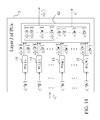
A PAM is a network of PUs (processing units) organized in one or more layers. A typical layer is shown in FIG. 14 . The feature vector input to layer l at time or numbering τ is denoted by xτ l-1, and the output from the layer at τ is denoted by x{yτ l}, which is a point estimate of the label of the feature vector xτ l-1. The symbols, yτ l and x{yτ l}, are defined and explained in detail below. A multilayer PAM without feedbacks is shown in FIG. 15 and is called a hierarchical PAM (HPAM). Note that the feature vector xτ 0 input to layer l of an HPAM is the exogenous feature vector xτ ex, and that for l>1, the feature vector xτ l-1 input to layer l is the output x{yτ l-1} from layer l-1. An example multilayer PAM with feedbacks is shown in FIG. 16 and is called a temporal HPAM (THPAM). Note that the feature vector xτ 0 input to layer 1 of an THPAM comprises the exogenous feature vector xτ ex and the feedbacks from the same or higher-ordered layers (e.g., x{yτ-1 1} and x{yτ-1 2} in FIG. 16 ) and that the feature vector xτ l-1 input to layer l comprises the output x{yτ l-1} from layer l-1 and feedbacks from the same or higher-ordered layers (e.g., xτ 2 comprises x{yτ 2}, x{yτ-1 5} and x{yτ-1 3} in FIG. 16 ). HPAMs and THPAMs are described in more detail in the subsection on “Multilayer and Recurrent Networks.” Before said subsection, this and the next 6 subsections describe essentially the PUs (processing units) in those networks. For notational simplicity, the superscript l-1 in xt l-1 and dependencies on l-1 or l in other symbols are usually suppressed in these 7 subsections when no confusion is expected.
Let xt, t=1, 2, . . . , denote a sequence of M-dimensional feature vectors xt=[xt1 . . . xtM]′, whose components are ternary numbers. The feature vectors xt, t=1, 2, . . . , are not necessarily different. The ternary entry xtm is called the m-th component of the feature vector xt. Let n=[n1 . . . nk]′ be a subvector [1 . . . M]′ such that n1< . . . <nk. The subvector xt(n)=[xtn 1 . . . xtn k ]′ is a feature subvector of the feature vector xt. n is called a feature subvector index (FSI), and xt(n) is said to be a feature subvector on the FSI n or have the FSI n. However, we stress that xt(n) is itself a feature vector. When a PU is discussed regardless of the layer of the PAM that the PU belongs, an input vector to the PU is referred to as a feature vector. Each PU is associated with a fixed FSI n and denoted by PU(n). Using these notations, the sequence of subvectors of xt, t=1, 2, . . . , that is input to PU(n) is xt(n), t=1, 2, . . . . An example of a group of ternary “pixels” that is identified with a feature subvector index n is shown in FIG. 3 . An FSI n of a PU usually has subvectors, n(u), u=1, . . . , U, on which subvectors xt(n(u)) of xt(n) are separately processed by PU(n) at first. The subvectors, n(u), u=1, . . . , U, are not necessarily disjoint, and their components are usually randomly selected from those of n. An example of such a subvector n(u) is shown in FIG. 3 and indicated by 46.
A PU in a PAM has a “receptive field” in the exogenous feature vector and a “receptive field” in the measurement vector. These receptive fields can be found by tracing the feedforward connections in the PAM backforward from a feature vector input to the PU (or the feature subvector index of the PU) to an exogenous feature vector (or the input terminals) of the PAM, and then tracing the transformation, that maps the measurement vector into the exogenous feature vector, backwards from the exogenous feature vector to the measurement vector. The components of the measurement vector that can be reached by this backward tracing from a PU to the exogenous feature vector and then to the measurement vector are called the “receptive field” of the PU in the measurement vector. The components of the exogenous feature vector that can be reached by this backward tracing from a PU to the exogenous feature vector are called the “receptive field” of the PU in the exogenous feature vector. The label of a feature vector input to a PU is the label of the corresponding components of the measurement vector in the receptive field of the PU in the measurement vector. The label of the corresponding components of the exogenous feature vector in the receptive field of the PU in the exogenous feature vector is also this label.
Let a label of the feature vector xt(n) be denoted by rt(n), which is an R-dimensional ternary vector. If R is 1, rt(n) is real-valued. All subvectors, xt(n(u)), u=1, . . . , U, of xt(n) share the same label rt(n). In supervised learning by PU(n), rt(n) is provided from outside the PAM, and in unsupervised learning by PU(n), rt(n) is generated by the PU itself.
The pairs (xt(n(u)), rt(n)), t=1, 2, . . . , are learned by the PU to form two of expansion correlation matrices, ECMs, D(n(u)), C(n(u)), A (n(u)), B(n(u)) on n(u). After the first T pairs are learned, these matrices are
where {hacek over (x)}t(n(u)) are orthogonal expansions of xt(n(u)), I=[1 . . . 1]′ with R components, Λ is a scaling constant that is selected to keep all numbers involved in an application of a PAM manageable, Wt(n(u), T) is a weight matrix, which is usually an diagonal matrix, diag(wt1(n(u), T) wt2(u), T) . . . wtR(n(u), T)), that is selected to place emphases on components of the label, place emphases on (xt(n(u)), rt(n)) of different numberings t, and keep the entries in the ECMs bounded. For example, Wt(n(u), T)=λT-t2−dim n(u)h(n(u))I, where λ (0<λ<1) is a forgetting factor, 2−dim n(u) eliminates the constant 2dim n(u) arising from {hacek over (x)}t(n(u)){hacek over (x)}t(n(u))=2dim n(u), and h(n(u)) assigns emphases to subvectors xt(n(u)) on n(u). There are many other possible weight matrices, depending on applications of the present invention.
Any two of the above four expansion correlation matrices (ECMs) can be obtained from the other two. We usually use D(n(u)) and C(n(u)) in this invention disclosure. They can be combined into one ECM [C′(n(u)) D′(n(u))]′. If Wt(n(u), T)=wt(n(u), T) I, where wt(n(u), T) is a real-valued function, all rows of C(n(u)) are equal, and only one needs to be stored.
ECMs, D(n(u)) and C(n(u)), can be adjusted to learn a pair (xτ(n(u)), rτ(n)). For example, if Wt(n(u), T)=λT-tI, the ECMs are adjusted as follows: If rτ(n) 0, D(n(u)) and C(n(u)) are replaced respectively with λD(n(u))+Λrτ(n){hacek over (x)}t(n(u)) and λC(n(u))+Λ{hacek over (x)}t′(n(u)), which are each a weighted sum of a ECM and rτ(n){hacek over (x)}t′(n(u)) or {hacek over (x)}t′(n(u)). If rτ(n)=0, then D(n(u)) and C(n(u)) are unchanged. Note that Wt(n(u), T) is a diagonal matrix, and C(n(u)) is a row vector here. This adjustment of the ECMs is shown in FIG. 5 .
If Wt(n(u), T)=I/√{square root over (T)}, the ECMs are adjusted as follows: If rτ(n)≠0, D(n(u)) and C(n(u)) are replaced respectively with (√{square root over (T)}D(n(u))+Λrτ(n){hacek over (x)}t′(n(u)))/√{square root over (T+1)} and (√{square root over (T)}C(n(u))+Λ{hacek over (x)}t′(n(u)))/√{square root over (T+1)}, which are each a weighted sum of a ECM and rτ(n){hacek over (x)}t′(n(u)) or {hacek over (x)}t′(n(u)), and √{square root over (T)} is replaced with √{square root over (T+1)}. If rτ(n)=0, then D(n(u)) and C(n(u)) are unchanged. Note that Wt(n(u), T) is a diagonal matrix, and C(n(u)) is a row vector here. This adjustment of the ECMs is shown in FIG. 6 .
Orthogonal expansions (OEs) {hacek over (x)}t(n(u)) and ECMs, D(n(u)), C(n(u)), A (n(u)), B(n(u)), u=1, . . . , U, are assembled into a general orthogonal expansion (GOE) {hacek over (x)}t(n) and general expansion correlation matrices (GECMs), D(n), C(n), A(n), B(n), for PU(n) (the PU on the feature subvector index n) as follows:
{hacek over (x)} t(n)=[{hacek over (x)} t′(n(1)){hacek over (x)} t′(n(2)) . . . {hacek over (x)} t′(n(U))]′ (7)
D(n)=[D(n(1))D(n(2)) . . . D(n(U))] (8)
C(n)=[C(n(1))C(n(2)) . . . C(n(U))] (9)
A(n)=[A(n(1))A(n(2)) . . . A(n(U))] (10)
B(n)=[B(n(1))B(n(2)) . . . B(n(U))] (11)
The GOE {hacek over (x)}t(n) and the GECMs, D(n) and C(n), are shown inFIG. 8 .
5.3 Representations of Probability Distributions
{hacek over (x)} t(n)=[{hacek over (x)} t′(n(1)){hacek over (x)} t′(n(2)) . . . {hacek over (x)} t′(n(U))]′ (7)
D(n)=[D(n(1))D(n(2)) . . . D(n(U))] (8)
C(n)=[C(n(1))C(n(2)) . . . C(n(U))] (9)
A(n)=[A(n(1))A(n(2)) . . . A(n(U))] (10)
B(n)=[B(n(1))B(n(2)) . . . B(n(U))] (11)
The GOE {hacek over (x)}t(n) and the GECMs, D(n) and C(n), are shown in
5.3 Representations of Probability Distributions
Let us define the symbols aτ(n(u)), bτ(n(u)), cτ(n(u)), dτ(n(u)) by
a τ(n(u)):=A(n(u)){hacek over (x)} τ(n(u)) (12)
b τ(n(u)):=B(n(u)){hacek over (x)} τ(n(u)) (13)
c τ(n(u)):=C(n(u)){hacek over (x)} τ(n(u)) (14)
d τ(n(u)):=D(n(u)){hacek over (x)} τ(n(u)) (15)
and the symbols aτ(n), bτ(n), cτ(n), dτ(n) by
a τ(n(u)):=A(n(u)){hacek over (x)} τ(n(u)) (12)
b τ(n(u)):=B(n(u)){hacek over (x)} τ(n(u)) (13)
c τ(n(u)):=C(n(u)){hacek over (x)} τ(n(u)) (14)
d τ(n(u)):=D(n(u)){hacek over (x)} τ(n(u)) (15)
and the symbols aτ(n), bτ(n), cτ(n), dτ(n) by
where {hacek over (x)}t(n) is a general orthogonal expansion (GOE) and D(n), C(n), A(n) and B(n) are general expansion correlation matrices (GECMs) for PU(n). It is easy to see that dτ(n(u))=2aτ(n(u))−cτ(n(u)), and dτ(n)=2aτ(n)−cτ(n).
To illustrate the use of aτ(n), bτ(n), cτ(n), dτ(n), two examples are given in the following: Example 1. Assume that xt(n) and xτ(n) are bipolar vectors, and Wt(n(u), T)=I/√{square root over (T)}. By Theorem 1, {hacek over (x)}t(n(u)) {hacek over (x)}τ(n(u))=0 or {hacek over (x)}t(n(u)){hacek over (x)}τ(n(u))=2dim n(u), depending on whether xk(n(u))≠xτ(n(u)) or xk(n(u))=xτ(n(u)). It follows that
a τj(n(u))=Λ2dimn(u) |G τj(n(u),+)|/√{square root over (T)} (20)
b τj(n(u))=Λ2dimn(u) |G τj(n(u),−)|/√{square root over (T)} (21)
G τj(n(u),+)={tε[0,T]|x t(n(u))=x τ(n(u)),r tj(n)=1} (22)
G τj(n(u),−)={tε[0,T]|x t(n(u))=x τ(n(u)),r tj(n)=−1} (23)
where |Gτj(n(u),+)| and |Gτj(n(u),−)| are the numbers of elements in the sets Gτj(n(u),+) and Gτj(n(u),−), respectively. If aτj(n(u))=bτj(n(u)) (i.e., cτj(n(u))=0, or cτj(n(u))≠0, but aτj(n(u))=bτj(n(u))), the ECMs for n(u) have no information or no preference about the value of the component rτj(n) of the label rτ(n) of the feature subvector xτ(n).
It follows that
(This shows that if dim n(u1)=dim n(u2)+k, then aτj(n(u1)) and cτj(n(u1)) are weighted 2k times as much as aτj(n(u2)) and cτj(n(u2)) in aτj(n) and cτj(n). This weighting can be changed by using Wt(n(u), T)=2−dim n(u)h(n(u))I/√{square root over (T)}.)
For simplicity and clarity, assume that dim n(u), u=1, . . . , U, are all the same. If cτj(n)≠0, then
can be viewed as a probability that rτj(n)=1. This probability is a subjective probability, because it is based on “experience” represented by the GECMs C(n) and A(n), or C(n) and D(n)=2A(n)−C(n), which are learned from (or constructed with) (xt(n(u)), rt(n)), t=1, 2, . . . , T.
Assume that all xt(n) and xτ(n) are bipolar binary vectors, and Wt(n(u), T)=λT-tI.
Assume further that dim n(u), u=1, U are all the same. Then if cτ(n)≠0,
can be viewed as a subjective probability that the label r (n)=1, based on the GECMs C(n) and A(n), or C(n) and D(n)=2A(n)−C(n), which are constructed with pairs (xt(n(u)), rt(n)), t=1, 2, . . . , T. The forgetting factor λ de-emphasizes past pairs gradually.
In both of the above examples, Wt(n(u), T) is a diagonal matrix with equal diagonal entries. In this case, all components cτj(n) of Cτ(n) are equal and all rows of C(n) are equal. Therefore, only one row of C(n), say C1(n), and one component of Cτ(n), say cτ1(n), are sufficient. If only C1(n) is used, it is also denoted by C(n).
In general, the ratio aτj(n)/cτj(n) can be viewed as a subjective probability that rτj(n)=1 based on the pairs (xt(n), rt(n)) that have been learned by PU(n) and the weight matrices Wt(n(u), T). All the statements concerning a probability in this invention disclosure are statements concerning a subjective probability, and the word “subjective” is usually omitted. If cτj(n)≠0, then aτj(n)/cτj(n) is the probability pτj(n) that the j-th component r (n) of the label rτ(n) of xτ(n) is +1 based on D(n) and C(n). If cτj(n)=0, then we set pτj(n)=1/2. The vector
p τ(n)=[p τ1(n)p τ2(n) . . . p τ R(n)]′
is a representation of a probability distribution of the label rτ(n) of the feature subvector xτ(n) input to PU(n). Since D(n)=2A(n)−C(n), if cτj(n)≠0, the ratio dτj(n)/cτj(n) is equal to 2pτj(n)−1. If cτj(n)=0, set 2pτj(n)−1=0. Denote 2pτj(n)−1 by yτj(n). Then the vector rτ(n)=2pτ(n)−I satisfies
and is also a representation of a probability distribution of the label rτ(n) of the feature subvector xτ(n). Here, I=[1 1 . . . 1]′.
5.4 Masking Matrices
Let a subvector xτ(n(u)) be a slightly different (e.g., corrupted, modified, deviated) version of xξ(n(u)), which is one of the subvectors, xt(n(u)), t=1, 2, . . . , T, stored in ECMs, D(n(u)) and C(n(u)) (or any two of the four ECMs, D(n(u)), C(n(u)), A (n(u)) and B(n(u)), on n(u)). Assume that xτ(n(u)) is very different from other subvectors stored in the ECMs. Since {hacek over (x)}ξ′(n(u)){hacek over (x)}τ(n(u))=0, the information stored in D(n(u)) and C(n(u)) about the label r (n) cannot be obtained from d(n(u))=D(n(u)){hacek over (x)}τ(n(u)) and c (n(u))=C(n(u)){hacek over (x)}τ(n(u)). This is viewed as failure of d (n(u)) and c (n(u)) or the ECMs to generalize or adequately generalize on xτ(n(u)). Because of property 2 in Theorem 1, if the corrupted, distorted and occluded components in xτ(n(u)) are set equal to zero, then the information stored in the ECMs about the label rξ(n) can be obtained in part from the remaining components of xτ(n(u)). This observation motivated masking matrices described in this section.
Let us denote the vector v=[v1 v2 . . . vn]′ with its i1-th, i2-th, . . . , and ii-th components set equal to 0 by v(i1 −, i2 −, . . . , ij −), where 1≦i1<i2< . . . <ij≦<n. For example, if v=[1 −1 −1 1]′, then v(2−, 4−)=[1 0 −1 0]′. Denoting the n-dimensional vector [1 1 . . . 1]′ by I and denoting the orthogonal expansion of v(i1 −, i2 −, . . . , ij −) by {hacek over (v)}(i1 −, i2 −, . . . , ij −), we note that v(i1 −, i2 −, . . . , ij −)=diag(I(i1 −, i2 −, . . . , ij −)) v and {hacek over (v)}(i1 −, i2 −, . . . , ij −)=diag({hacek over (I)}(i1 −, i2 −, . . . , ij −)) {hacek over (v)}, were {hacek over (v)}(i1 −, i2 −, . . . , ij −) and {hacek over (I)}(i1 −, i2 −, . . . , ij −) denote the orthogonal expansions of v(i1 −, i2 −, . . . , ij −) and I(i1 −, i2 −, . . . , ij −) respectively (not the orthogonal expansions of v and I with their i1-th, i2-th, . . . , and ij-th components set equal to 0).
Using these notations, a feature subvector x (n(u)) with its i1-th, i2-th, . . . , and ij-th components set equal to 0 is xt(n(u)) (i1 −, i2 −, . . . , ij −), and the orthogonal expansion of xt(n(u)) (i1 −, i2 −, . . . , ij −) is diag({hacek over (I)}(i1 −, i2 −, . . . , ij −)){hacek over (x)}t(n(u)). Hence, the matrix diag({hacek over (I)}(i1 −, i2 −, . . . , ij −), as a matrix transformation, sets the i1-th, i2-th, . . . , and ij-th components of xt(n(u)) equal to zero in transforming {hacek over (x)}t(n(u)) (i.e., diag({hacek over (I)}(i1 −, i2 −, . . . , ij −)){hacek over (x)}t(n(u))). Therefore, diag({hacek over (I)}(i1 −, i2 −, . . . , ij −)) is called a masking matrix.
An important property of the masking matrix diag({hacek over (I)}(i1 −, i2 −, . . . , ij −)) is the following: If
diag({hacek over (I)}(i 1 − ,i 2 − , . . . ,i j −)){hacek over (x)} t(n(u))=diag({hacek over (I)}(i 1 − ,i 2 − , . . . ,i j −)){hacek over (x)}τ(n(u))
then
{hacek over (x)} t(n(u))diag({hacek over (I)}(i 1 − ,i 2 − , . . . ,i j −)){hacek over (x)} τ(n(u))=2dimn(u)-j.
If
diag({hacek over (I)}(i 1 − ,i 2 − , . . . ,i j −)){hacek over (x)} t(n(u))=diag({hacek over (I)}(i 1 − ,i 2 − , . . . ,i j −)){hacek over (x)}τ(n(u))
then
{hacek over (x)} t(n(u))diag({hacek over (I)}(i 1 − ,i 2 − , . . . ,i j −)){hacek over (x)} τ(n(u))=2dimn(u)-j.
If
-
- diag({hacek over (I)}(i1 −,i2 −, . . . , ij −)) {hacek over (x)}t(n(u))≠diag ({hacek over (I)}(i1 −, i2 −, . . . , ij −)) {hacek over (x)}τ(n(u)) then (n(u))diag({hacek over (I)}(i1 −, i2 −, . . . , ij −)) {hacek over (x)}τ(n(u))=0.
Using this property, we combine all such masking matrices that set less than or equal to a selected positive integer J (n(u)) of components of xt(n(u)) equal to zero into the following masking matrix
where 2j is used to compensate for the
Let us denote M(n(u)) by M here for abbreviation. Note that for j=1, . . . , R, we have the following:
If Cj(n(u)){hacek over (x)}τ(n(u))≠0, then
D j(n(u)){hacek over (x)} τ(n(u))≈D j(n(u))M{hacek over (x)} τ( n(u))
C j(n(u)){hacek over (x)} τ(n(u))≈C j(n(u))M{hacek over (x)} τ( n(u))
A j(n(u)){hacek over (x)} τ(n(u))≈A j(n(u))M{hacek over (x)} τ( n(u))
B j(n(u)){hacek over (x)} τ(n(u))≈B j(n(u))M{hacek over (x)} τ( n(u))
D j(n(u)){hacek over (x)} τ(n(u))≈D j(n(u))M{hacek over (x)} τ( n(u))
C j(n(u)){hacek over (x)} τ(n(u))≈C j(n(u))M{hacek over (x)} τ( n(u))
A j(n(u)){hacek over (x)} τ(n(u))≈A j(n(u))M{hacek over (x)} τ( n(u))
B j(n(u)){hacek over (x)} τ(n(u))≈B j(n(u))M{hacek over (x)} τ( n(u))
If Cj(n(u)){hacek over (x)}τ(n(u))=0, but
then
If Cj(n(u)) xτ(n(u))=0,
but
then
Continuing in this manner, it is seen that Dj(n(u)) M{hacek over (x)}τ(n(u)), Cj(n(u)) M{hacek over (x)}τ(n(u)), Aj(n(u)) M{hacek over (x)}τ(n(u)), Bj(n(u)) M{hacek over (x)}τ(n(u)) always use the greatest number of uncorrupted, undeviated or unmodified components of xτ(n(u)) in estimating dτj(n(u)), cτj(n(u)), aτj(n(u)), bτj(n(u)), respectively.
Corresponding to {hacek over (x)}t(n), D(n), C(n), A(n), B(n) defined in (7), (8), (9), (10), (11), a general masking matrix is defined as follows:
M(n)=diag[M(n(1))M(n(2)) . . . M(n(U))] (27)
where the right side is a matrix with M(n(u)), u=1, 2, . . . , U, as diagonal blocks and zero elsewhere. M(n) is shown inFIG. 9 .
M(n)=diag[M(n(1))M(n(2)) . . . M(n(U))] (27)
where the right side is a matrix with M(n(u)), u=1, 2, . . . , U, as diagonal blocks and zero elsewhere. M(n) is shown in
If the masking matrix M(n(u)) is used, the symbols aτ(n(u)), bτ(n(u)), cτ(n(u)), dτ(n(u)) are defined as follows:
a τ(n(u)):=A(n(u))M(n(u)){hacek over (x)} τ(n(u)) (28)
b τ(n(u)):=B(n(u))M(n(u)){hacek over (x)} τ(n(u)) (29)
c τ(n(u)):=C(n(u))M(n(u)){hacek over (x)} τ(n(u)) (30)
d τ(n(u)):=D(n(u))M(n(u)){hacek over (x)} τ(n(u)) (31)
If the masking matrix M(n) is used, the symbols aτ(n), bτ(n), Cτ(n), dτ(n) are defined as follows:
where {hacek over (x)}t(n) is a general orthogonal expansion (GOE) and D(n), C(n), A(n) and B(n) are general expansion correlation matrices (GECMs) for PU(n). It follows that
It is easy to see that dτ(n(u))=2aτ(n(u))−cτ(n(u)), and dτ(n)=2aτ(n)−cτ(n). If cτj(n)=0, then we set dτj(n)/cτj(n)=0. If cτj(n)≠0, then dτj(n)/cτj(n)=2pτj(n)−1, where pτj(n) is the probability that the j-th component rτj(n) of the label rτ(n) of xτ(n) is +1 based on D(n) and C(n). It follows that
2p τ(n)−1=[d τ1(n)/c τ1(n)d τ2(n)d τ2(n)/c τ2(n) . . . d τR(n)/c τR(n)]′ (40)
is a representation of a probability distribution of the label rτ(n) of xτ(n).
An estimation means for generating this representation of a probability distribution is shown in FIG. 10 : For j=1, 2, . . . , R, if cτj(n)=0, then set yτj(n)=0, else set yτj(n)=dτj(n)/cτj(n). The output of the estimation means is yτ(n)=[yτ1(n) yτ2(n) . . . yτR(n)]′, which is a representation 2p τ(n)−1 of a probability distribution of the label rτ(n) of xτ(n).
5.5 Conversion of Probabilities into Ternary Numbers
In a multilayer PAM, a feature vector into layer l is a ternary vector denoted by xt l-1, where t denotes a numbering of the feature vector or a time instant. In this subsection, two methods of converting a representation of a probability distribution, y τ(n)=[y τ1(n)y τ2(n) . . . y τ R(n)]′, generated by a PU (processing unit) into a ternary vector are described. Recall yτk(n)=2pτk(n)−1, where Pτk(n) is a probability that rτk(n) is +1. pτ(n)=[pτ1(n) pτ2(n) . . . pτR(n)]′ is an alternative representation of probability distribution of pτ(n). yτ(n) and pτ(n) are related by yτ(n)=2pτ(n)−I.
5.6 Processing Units and Supervised/Unsupervised Learning
An example PU(n) (processing unit on a feature subvector index n) is shown in FIG. 13 . The PU comprises expansion means 2, estimation means 54, conversion means 13, adjustment means 9 and storage means 56. A PU has essentially two functions, retrieving an estimate of the label of a feature subvector from the memory (i.e., ECMs or GECMs) and learning a feature subvector and its label that is either provided from outside the PU (in supervised learning) or generated by itself (in unsupervised learning). In performing retrieval, a feature subvector xτ(n) on the FSI n is first expanded into a general orthogonal expansion {hacek over (x)}τ(n) by the expansion means 2. {hacek over (x)}τ(n) is then processed by the estimation means, using the general expansion correlation matrices, C(n) and D(n), from the storage means 56, into a representation of a probability distribution yτ(n) of the label of xτ(n). The conversion means converts yτ(n) into a ternary vector x{yτ(n)}, which is an output of the PU. If a representation of a probability distribution of xτ(n) is needed for use outside the PU, yτ(n) is also output by the PU. The dashed line in the arrow 55 indicates “output as needed.” yτ(n) and x{yτ(n)} are the products of retrieval.
C(n) and D(n) model the synaptic weights in a cortex. The estimation means and conversion means constitute a processing node, which models a group of R neurons in a cortex.
Recall that a PU in a PAM has a “receptive field” in the exogenous feature vector and a “receptive field” in the measurement vector. These receptive fields can be found by tracing the feedforward connections in the PAM backforward from a feature subvector input to the PU (or the feature subvector index of the PU) to an exogenous feature vector (or the input terminals) of the PAM, and then tracing the transformation, that maps the measurement vector into the exogenous feature vector, backward from the exogenous feature vector to the measurement vector. The components of the measurement vector that can be reached by this backward tracing from a PU to the exogenous feature vector and then to the measurement vector are called the “receptive field” of the PU in the measurement vector. The components of the exogenous feature vector that can be reached by this backward tracing from a PU to the exogenous feature vector are called the “receptive field” of the PU in the exogenous feature vector. The label of a feature vector input to a PU is the label of the corresponding components of the measurement vector in the receptive field of the PU in the measurement vector. The label of the corresponding components of the exogenous feature vector in the receptive field of the PU in the exogenous feature vector is also this label
If a label rτ(n) of xτ(n) from outside the PU is available for learning, supervised learning can be performed by the PU. In the supervised learning mode, the label rτ(n) is received through a lever represented by a thick solid line with a solid dot in the position 48 by a general expansion correlation matrix (GECM) adjustment means 9, which receives also {hacek over (x)}τ(n) and uses a method of adjusting ECMs such as those depicted in FIG. 5 and FIG. 6 and assembles the resultant ECMs
C(n)=[C(n(1))C(n(2)) . . . C(n(U))]
D(n)=[D(n(1))D(n(2)) . . . D(n(U))]
These C(n) and D(n) are then stored, after a one-numbering delay (or a unit-time delay) 33, in thestorage 56, from which they are sent to the estimation means 54. The one-numbering delay is usually a time delay that is long enough for the estimation means to finish using current C(n) and D(n) in generating and outputting yτ(n), but short enough for getting the next C(n) and D(n) generated by the adjustment means available for the estimation means to use for processing the next orthogonal expansion or general orthogonal expansion from the expansion means.
C(n)=[C(n(1))C(n(2)) . . . C(n(U))]
D(n)=[D(n(1))D(n(2)) . . . D(n(U))]
These C(n) and D(n) are then stored, after a one-numbering delay (or a unit-time delay) 33, in the
Supervised learning means of the PU comprises adjustment means 9 for adjusting at least one GECM (general expansion correlation matrix) by receiving a GOE (general orthogonal expansion) {hacek over (x)}τ(n) generated by expansion means 2 and a label rτ(n) of xτ(n) provided from outside the PAM and replacing said at least one GECM with a weighted sum of said at least one GECM and a product of said label rτ(n) and the transpose of said GOE {hacek over (x)}τ(n).
If a label rτ(n) of xτ(n) from outside the PU is unavailable, unsupervised learning can be performed by the PU. In this case, the lever (shown in position 48 in FIG. 13 ) should be in the position 50. The feature subvector xτ(n) is first processed by the expansion means 2, estimation means 54, conversion means 13 as in performing retrieval described above. The resultant ternary vector x{yτ(n)} is received, through the lever in position 50, and used by the adjustment means 9 as the label rτ(n) of xτ(n). The adjustment means 9 uses rτ(n)=x{yτ(n)} and {hacek over (x)}τ(n) to adjust C(n) and D(n) and store the resultant C(n) and D(n) in the storage 56 after a one-numbering delay (or a unit-time delay) 33.
It is sometimes expensive or impossible to provide labels to feature subvectors yτ(n) especially for PUs in lower layers of a PAM. If a label rτ(n) of xτ(n) is not provided from outside the PU(n), unsupervised learning can be performed by the PU. In this case, the lever in position 48 should be switched to the position 50. The ternary vector x{yτ(n)} generated by the conversion means in performing retrieval is received and used by the adjustment means 9 as the label rτ(n) of xτ(n). As in supervised learning described above, the adjustment means 9 uses rτ(n) and Xτ(n) to adjust C(n) and D(n) and store the resultant C(n) and D(n) in the storage 56.
This unsupervised learning method is consistent with the Hebb rule of learning: The synaptic weight between two neurons is increased if the neurons fire at the same time, and the synaptic weight decreases otherwise. Nevertheless, the orthogonal expansion 2 of xτ(n(u)), the masking matrix M(n(u)) 11 a, the conversion 13 and the estimation 54 used in this invention are new.
If a feature subvector xτ(n) or a slightly different version of it has not been learned by PU(n), and C(n) {hacek over (x)}τ(n)=0, then yτ(n)=0 and pτ(n)=(½)I, where I=[1 1 . . . 1]′. The conversion means shown in FIG. 11 converts yτ(n) into a purely random label rτ(n)=x{yτ(n)}, with the probability that x{yτk(n)}=+1 being equal to ½ for k=1, 2, . . . , R. Once this xτ(n) has been learned and stored in C(n) and D(n), if xτ(n) is input to PU(n) and to be learned without supervision for the second time, then x{yτ(n)}=rτ(n) and one more copy of the pair (xτ(n), rτ(n)) is included in C(n) and D(n). Note that the conversion means 13 b shown in FIG. 12 converts yτ(n)=0 into x{yτk(n)}=0. Hence, this conversion means 13 b in FIG. 12 cannot be used for unsupervised learning.
Assume a feature subvector xτ(n) is a noise vector and is given a label in unsupervised learning by PU(n). If the noise vector is not repeatedly fed to the PU, as is usually the case, this noise vector and other noise vectors distruct themselves in C(n) and D(n).
If no learning is to be performed by the PU, the lever represented by a thick solid line with a solid dot is placed in the position 49, through which 0 is sent as the label rτ(n) of xτ(n) to the adjustment means, which then keeps C(n) and D(n) unchanged or stores the same C(n) and D(n) in the storage 56 after a one-numbering delay (or a unit time delay).
There are three types of PU:
-
- 1. Supervised PU. This type of PU is only capable of performing supervised learning. In a PU of this type, the position, 50, in
FIG. 13 does not exist. If a label rτ(n) of xτ(n) from outside the PU is available and wanted for learning, the lever represented by a thick solid line with a solid dot is placed in theposition 48, through which rτ(n) is sent to the adjustment means 9. If rτ(n) is not available or wanted for learning, the lever is placed in theposition 49, through which 0 is sent to the adjustment means 9. A condition under which learning is not wanted is given below. It is understood that the “lever” is simply a symbol used here to explain which “label” to use by the adjustment means 9. - 2. Unsupervised PU. This type of PU is only capable of performing unsupervised learning. In a PU of this type, the position, 48, in
FIG. 13 does not exist. If unsupervised learning is wanted, then the output x{yτ(n)} is used as a label rτ(n) of xτ(n), and the lever represented by a thick solid line with a solid dot is placed in theposition 50, through which rτ(n) is sent as to the adjustment means 9. If no learning is wanted, the lever is placed in theposition 49, through which 0 is sent to the adjustment means 9. A condition under which learning is not wanted is given below. It is understood that the “lever” is simply a symbol to explain which “label” to use by the adjustment means 9. - 3. Supervised/Unsupervised PU. This type of PU is capable of performing both supervised and unsupervised learning. In a PU of this type, all the three positions, 48, 49 and 50, in
FIG. 13 coexist. If a label rτ(n) of xτ(n) from outside the PU is available and wanted for learning, the lever represented by a thick solid line with a solid dot is placed in theposition 48. If a label rτ(n) of xτ(n) from outside the PU is unavailable, but expected to become available, and yτ(n) generated by the PU's estimation means in its performing retrieval mode is a zero vector or sufficiently close to it by some criterion, then the lever is placed in theposition 49 and no learning is performed. This avoids generating and establishing a randomly selected label in unsupervised learning, which may turn out to be difficult to “unlearn” through supervised learning. If a label rτ(n) of xτ(n) from outside the PU is unavailable, yτ(n) generated by the PU's estimation means in its performing retrieval is neither a zero vector nor sufficiently close to it by some criterion, and unsupervised learning for strengthening learned the knowledge stored in the GECMs (general expansion correlation matrices) or ECMs in the PU is wanted, then the lever is placed in theposition 50 and unsupervised learning is performed. A condition under which learning is not wanted is given below.
- 1. Supervised PU. This type of PU is only capable of performing supervised learning. In a PU of this type, the position, 50, in
A condition under which the lever is placed in the position 49 and no learning is performed is the following: If yτ(n) generated by a PU's estimation means in retrieving is a bipolar vector or sufficiently close to a bipolar vector by some criterion, which indicates that the input feature subvector xτ(n) is adequately learned, then the lever is placed in the position 49 and no learning is performed. This avoids “saturating” the expansion correlation matrices with one feature subvector and its label.
It is understood that the “lever” and “lever positions” are simply a symbol used here to explain which label to use by the adjustment means 9. In application of the present invention, the “lever” and “lever positions” are implemented usually by software to select among supervised learning, unsupervised learning and no learning. Of course, hardware implementation is also possible.
Note that the learning methods for the three types of PE described above are valid for both batch learning and online learning and jointly or separately, and are suitable for semi-autonomous or autonomous learning. Note also that a PU in a PAM usually has a “receptive field” in the measurement vectors which can be found by tracing the feedforward connections in the PAM backforward from the feature subvectors input to the PU (or the feature subvector index of the PU) to the exogenous feature vectors (or the input terminals) of the PAM, and tracing the transformation, that maps the measurement vectors into exogenous feature vectors, backforward from exogenous feature vectors to measurement vectors. For supervised learning, a feature vector input to a PU is usually assigned the same label as (or is assigned a translation of) the label of the subvector of the measurement vector that appears in the receptive field of the PU. It is understood that there are other ways to assign a label to a feature subvector for supervised learning.
5.7 Learning to Recognize Rotated, Translated or Scaled Patterns
In this subsection, we describe methods for PUs (processing units) to learn to recognize rotated, translated and scaled patterns. The methods can be modified for PUs to learn to recognize trans-lated and scaled temporal patterns such as speech and music. The methods are valid for both supervised and unsupervised learning. Therefore, labels rt(n) to be referred to may be provided from outside the PAM in supervised learning or generated by the PUs in unsupervised learning for the three types of PU, supervised PUs, unsupervised PUs and supervised/unsupervised PUs described at the end of the last Subsection.
It is assumed in this subsection that feature vectors are arrays of ternary pixels. Other types of feature vector must be converted into arrays of ternary pixels for the methods to be described to apply. For example, an image with 8-bit pixels may be converted by using a pseudo-random number generator to generate a bipolar pulse train for each pixel whose average pulse rate (i.e., the rate of +1 pulse) is proportional to 8-bit light intensity of the pixel. Another way to convert an image with 8-bit pixels is to replace an 8-bit pixel with 3 bipolar 2-bit pixels placed at the same location in considering rotation, translation and scaling. After conversion, at any instant of time, the feature vector is an array of ternary pixels.
Locations of ternary pixels in an array are assumed to be dense relative to the locations of the pixels selected as components of a feature subvector xt(n) input to a PU. We identify the FSI (feature subvector index) n of a feature subvector with the locations of the pixels in xt(n). In other words, the components of n are also the numberings of the locations of the pixels included as components of xt(n).
Consider a PU with an FSI n shown in FIG. 3 and FIG. 17 a. Imagine a thin rubber rectangle with small holes at the locations n of the pixels of the feature subvector with the FSI n. We translate the rectangle in some directions (e.g., 0, 15, 30, 45, . . . , 330, 345 degrees) (FIG. 17 b) a number of steps (e.g., 0, 1, 2, . . . ), rotate the rectangle clockwise and counterclockwise a number (e.g., 0, 1, 2, . . . ) of angles (e.g., 0, 5, 10, 15 degrees) at each translation (FIG. 17 c), and expand and compress the rubber rectangle uniformly for a number of times (e.g., 0, 1, 2, . . . ) at each translation for some percentages (e.g., 0%, 5%, 10%, . . . ) (FIG'S. 17 d and 17 e), to obtain other feature subvector indices of the same dimensionality as n. Note that in using the rubber rectangle to determine an FSI, if a hole in the rubber rectangle contains more than one pixel in the image, the one nearest to the center of the hole is included in the FSI.
Let Ω(n)={w(i), i=1, . . . , |Ω(n)|} be a set of FSIs w(i) identified with such rotations, translations, and scalings of n including n. Ω(n) is called a rotation/translation/scaling (RTS) suite of n, and |Ω(n)| denotes the number of elements in Ω(n). Note that an RTS suite may contain only rotations, or only translations, or only scalings, or a combination thereof. (Notice the digit 0 in the parentheses (e.g., 0, 1, 2, . . . ) in the last paragraph. It indicates a rotation, a translation, or a scaling that is the feature subvector itself.) As a special case of Ω(n), there is only one element in the set Ω(n) that is n itself. In this special case, |Ω(n)|=1.
Although w(i) is a rotation, translation, or scaling of n, this dependence on n is not indicated in the symbol w(i) for notational simplicity. As n is rotated, translated or scaled into w(i), n(u) as a subvector of n is rotated, translated or scaled into a subvector of w(i). This subvector of w(i) is denoted by n(u,w(i)). The set {n(u,w(i)), i=1, . . . , |Ω(n)|} of such subvectors of w(i), i=1, . . . , |Ω(n)|, is denoted by Ω(n(u)) and called a rotation/translation/scaling (RTS) suite of n(u). Note that |Ω(n(u))|=|Ω(n)|. The set {xt(n(u,w(i))), i=1, . . . , |Ω(n)|}, which is also denoted by {xt(n(u,w)), wεΩ(n)}, is called the rotation/translation/scaling (RTS) suite of xt(n(u)) on Ω(n(u)). In generating and summing orthogonal expansions on an RTS suite Ω(n(u)), elements in the RTS suite of xt(n(u)) on Ω(n(u)) first go through orthogonal expansion 1. The resultant orthogonal expansions {hacek over (x)}t(n(u,w(i))) are then added up to form the sum τwεΩ(n){hacek over (x)}t(n(u,w)) on the RTS suite Ω(n(u)) of n(u) (FIG. 18 ).
In both the supervised learning and unsupervied learning, the subvectors, xt(n(u,w)), w E Ω(n), on Ω(n(u)) are assigned the label rt(n) of xt(n). ECMs (expansion correlation matrices), C(n(u)), D(n(u)), A (n(u)) and B(n(u)), on Ω(n(u)) are defined by
Definitions of C(n(u)) and D(n(u)) are shown in
C(n(u)) and D(n(u)) for the weight matrix Wt(n(u), T)=λT-tI can be adjusted to learn a pair (xt, rt(n)), where λ is a forgetting factor, and Λ is a scaling constant. If rτ(n)≠0, D(n(u)) and C(n(u)) are replaced respectively with λD(n(u))+Λrτ(n) τwεΩ(n){hacek over (x)}t′(n)(u,w)) and λC(n(u))+ΛτwεΩ(n){hacek over (x)}t′(n(u,w)), which are each a weighted sum of a ECM and rτ(n) τwεΩ(n){hacek over (x)}t′(n(u,w)) or τwεΩ(n){hacek over (x)}t′(n(u,w)). If rτ(n)=0, then D(n(u)) and C(n(u)) are unchanged. Note that Wt(n(u), T) is a diagonal matrix, and C(n(u)) is a row vector here. This adjustment of the ECMs is shown in FIG. 20 .
If Wt(n(u), T)=I/√{square root over (T)}, the ECMs are adjusted as follows: If rτ(n)≠0, D(n(u)) and C(n(u)) are replaced with (√{square root over (T)}D(n(u))+Λrτ(n){hacek over (x)}t′(n(u)))/√{square root over (T+1)} and (√{square root over (T)}C(n(u))+Λ{hacek over (x)}t′(n(u)))/√{square root over (T+1)}, which are each a weighted sum of a ECM and rτ(n)τwεΩ(n){hacek over (x)} t′(n(u,w)) or ΣwεΩ(n){hacek over (x)}t′(n(u,w)), and √{square root over (T)} is replaced with √{square root over (T+1)}. If rτ(n)=0, then D(n(u)) and C(n(u)) are unchanged. Note that Wt(n(u), T) is a diagonal matrix, and C(n(u)) is a row vector here. This adjustment of the ECMs is shown in FIG. 21 .
Sums τwεΩ(n){hacek over (x)}t(n(u,w)) of orthogonal expansions (OEs), and ECMs, D(n(u)), C(n(u)), A(n(u)), B(n(u)), u=1, . . . , U, are respectively assembled into a general orthogonal expansion (GOE) {hacek over (x)}t(n) and general expansion correlation matrices (GECMs), D(n), C(n), A(n), B(n), for PU(n) (the PU on the feature vector n) as follows:
{hacek over (x)} t′(n,Ω)=[ΣwεΩ(n) {hacek over (x)} t′(n(1,w)) . . . ΣwεΩ(n) {hacek over (x)} t′(n(2,w))])) (45)
D(n)=[D(n(1))D(n(2)) . . . D(n(U))] (46)
C(n)=[C(n(1))C(n(2)) . . . C(n(U))] (47)
A(n)=[A(n(1))S(n(2)) . . . A(n(U))] (48)
B(n)=[B(n(1))B(n(2)) . . . B(n(U))] (49)
where these definitions of {hacek over (x)}t(n,Ω), D(n) and C(n) are shown inFIG. 22 .
{hacek over (x)} t′(n,Ω)=[ΣwεΩ(n) {hacek over (x)} t′(n(1,w)) . . . ΣwεΩ(n) {hacek over (x)} t′(n(2,w))])) (45)
D(n)=[D(n(1))D(n(2)) . . . D(n(U))] (46)
C(n)=[C(n(1))C(n(2)) . . . C(n(U))] (47)
A(n)=[A(n(1))S(n(2)) . . . A(n(U))] (48)
B(n)=[B(n(1))B(n(2)) . . . B(n(U))] (49)
where these definitions of {hacek over (x)}t(n,Ω), D(n) and C(n) are shown in
How a GOE (general orthogonal expansion) {hacek over (x)}t(n,Ω) on an RTS suite Ω(n), is generated is shown in FIG. 23 .
5.8 Processing Units for Recognizing Rotated, Translated and Scaled Patterns
An example PE (processing unit) that is capable of recognizing rotated, translated and scaled images of causes (e.g., objects) is given in FIG. 24 . Notice that FIG. 24 is essentially the same as FIG. 13 except that the input feature subvector xτ(n), box 2 (expansion means for generating GOEs on n) and box 9 (adjustment means for adjusting GECMs) in FIG. 13 are respectively replaced with xτ, box 18 (expansion means for generating GOEs on n and GOEs on Ω(n)) and box 9 (adjustment means for adjusting GECMs on Ω(n)) in FIG. 24 .
The feature vector xτ that is input to PE in FIG. 24 is first used 18 to generate the GOE (general orthogonal expansion) {hacek over (x)}τ(n) defined in (7) (FIG. 8 ) and GOE {hacek over (x)}t(n,Ω) on the RTS suite Ω(n) defined in (45) (FIG. 22 ). The GOE {hacek over (x)}τ(n) is then sent to the estimation means 54, and the GOE {hacek over (x)}t(n,Ω) on Ω(n) is sent to the adjustment means 9.
Responsible to {hacek over (x)}τ(n,Ω) and the label rτ(n), which is provided from outside the PU in supervised learning or generated by the conversion means 13, the adjustment means 9 adjusts GECMs (general expansion correlation matrices) D(n) and C(n) on Ω(n), which are defined in (46) and (47) (FIG. 22 ). The adjustment is performed by replacing D(n(u)) with a weighted sum of D(n(u)) and rτ(n) τwεΩ(n){hacek over (x)}τ′(n(u,w)) and replacing C(n(u)) with a weighted sum of C(n(u)) and IτwεΩ(n){hacek over (x)}τ′(n(u,w)). If Wt(n(u),T)=wt(n(u),T) I, all rows of C(n(u)) are the same and only one row is needed to represent C(n(u)), and IΣwεΩ(n){hacek over (x)}τ′(n(u,w)) used for adjusting C(n(u)) can be replaced with IΣwεΩ(n){hacek over (x)}τ′(n(u,w)). Two examples of the adjustment means are given in FIG. 20 and FIG. 21 .
Other than the foregoing differences between the PUs in FIG. 13 and FIG. 24 , these PUs' estimation means 54, conversion means 13, supervised learning means 48, 9, unsupervised learning means 49, 9, storage 56 of the GECM [C′(n) D′ (n)]′ function in much the same way.
If more capability of recognizing rotated, translated and scaled images is required of the PU, an additional RTS suite, Ω1(n), is used. Instead of generating the GOE {hacek over (x)}τ(n), another GOE {hacek over (x)}t(n,Ω1) on the RTS suite Ω1(n) is generated and sent to the estimation means 54. In generating a representation yτ(n) of a probability distribution, {hacek over (x)}t(n,Ω1) is used here in box 54. Such a PU is shown in FIG. 25 .
There are also three types of PU, supervised PUs, unsupervised PUs and supervised/unsupervised PUs as discussed at the end of the Subsection on “Processing Units and Supervised/Unsupervised Learning.”
5.9 Multilayer and Recurrent Networks
An embodiment of the present invention comprises at least one layer of PUs, which are discussed in the Subsection on “Processing Units and Supervised/Unsupervised Learning” and the Subsection on “Processing Units for Recognizing Rotated, Translated and Scaled Images.” A typical layer, layer l, is shown in FIG. 14 . A feature vector xτ 0 input to layer 1 comprises an exogenous feature vector xτ ex input to the network. In this Subsection, l is used in superscripts to emphasize dependency on layer numberings such as l-1 and l.
There are at least one PU in layer l (5 in FIG. 14 ). The PUs in layer l have FSIs (feature subvector indices) denoted by 1 l, 2 l, . . . , Nl. Upon receiving a feature vector xτ l-1 by layer l, the feature subvectors, xτ l-1(1 l), xτ l-1(2 l), . . . , xτ l-1(Nl), are formed and processed by the PUs (15 in FIG. 14 ), PU(1 l), PU(2 l), . . . , PU(Nl) to generate x {yτ l(1 l)}, x{yτ l(2 l)}, . . . , x{yτ l(Nl)}, respectively. These ternary vectors are then assembled (42 in FIG. 14 ) into the output vector x{yτ l} of layer l. If needed, yτ l(1 l), yτ l(2 l), . . . , yτ l(Nl), are also assembled and output from layer l.
If an embodiment of the present invention comprises a plurality of layers (5 in FIG. 14 ) with only feedforward connections and no feedback connections as shown in FIG. 15 , the embodiment is called a hierarchical probabilistic associative memory (HPAM). The feature vector input to layer l=1 is the exogenous feature vector xτ ex input to the embodiment. If l>1, the components of a feature vector xτ l-1 input to layer l are components of ternary vectors, x{yτ l-1(1 l-1)}, x{yτ l-1(2 l-1)}, . . . , x{yτ l-1(Nl-1)}, generated by PU(1 l-1), PU(2 l-1), . . . , PU(Nl-1) in layer l-1.
If the above embodiment further comprises feedback connections, it is called a temporal hierarchical probabilistic associative memory (THPAM). An example THPAM is shown in FIG. 16 . Two types of feedback connections are shown, namely same-layer feedback connections (371, 372, 373, 374 in FIG. 16 ) and 1-layer feedback connections (352, 353, 354 in FIG. 16 ). The components of a feature vector xτ l-1 input to layer l at time (or with numbering) τ comprise components of ternary vectors generated by PUs in layer l-1 and generated at a previous time (or for a feature vector with a lower numbering) by PUs in the same layer l or PUs in higher-ordered layers with layer numberings l+k for some positive integers k. Example 1: The components of the feature vector xτ 2 input to layer 3 in the example THPAM are components of x{yτ 2} generated by PUs in layer 2 and components of x{yτ-1 4} and x{yτ-1 3}, which are generated by PUs in layer 4 and layer 3 for the exogenous feature vector xτ-1 ex input to the THPAM at time τ−1. Note that the small boxes 33 enclosing 1 in FIG. 16 are delay devices. Example 2: The feature vector xτ 0 input to layer 1 comprises the exogenous feature vector xτ ex and the feedbacked ternary vectors (e.g., x{yτ-1 2} and x{yτ-1 1} in FIG. 16 ).
Once an exogenous feature vector is received by an HPAM or THPAM, the PUs perform functions of retrieving and/or learning from layer to layer starting with layer 1, the lowest-ordered layer. After the PUs in the highest-ordered layer, layer L, complete performing their functions, the HPAM or THPAM is said to have completed one round of retrievings and/or learnings (or memory adjustments).
It is understood that an HPAM may further comprises feedforward connections with delay devices, and that the delay devices in a THPAM or an HPAM may effect delays of more than one unit of time (or one numbering) or even different lengths.
5.10 Processing Units for Recognizing Extensively Translated Images
Assume that FSIs, 1 l, 2 l, . . . , Nl, in layer l are translations of one another, and hence so are their subvectors 1 l/(u), 2 l (u), . . . , Nl(u), for each u=1, . . . , Ul, where Ul denotes the number of FSIs in layer l. Recall that the GOE (general orthogonal expansion) {hacek over (x)}τ l-1(n) defined in (7) (FIG. 8 ) and the GOE {hacek over (x)}t l-1 (n,Ω) on the RTS suite Ω(n) are defined in (45) (FIG. 22 ). The general orthogonal expansion on n1 is
{hacek over (x)} t l-1(n l)=[{hacek over (x)} t l-1′(n l(1)){hacek over (x)} t l-1′(n l(2)) . . . {hacek over (x)} t l-1′(n l(U))]′
and the general orthogonal expansion on Ω(nl) is
{hacek over (x)} t l-1′(n l,Ω)=[ΣwεΩ(nl ) {hacek over (x)} t l-1′(n l(1,w)) . . . ΣwεΩ(n) {hacek over (x)} t l-1′(n l(2,w))]
Here, l is used in superscripts to emphasize dependency on layer l-1 or layer l.
{hacek over (x)} t l-1(n l)=[{hacek over (x)} t l-1′(n l(1)){hacek over (x)} t l-1′(n l(2)) . . . {hacek over (x)} t l-1′(n l(U))]′
and the general orthogonal expansion on Ω(nl) is
{hacek over (x)} t l-1′(n l,Ω)=[ΣwεΩ(n
Here, l is used in superscripts to emphasize dependency on layer l-1 or layer l.
To enable recognition of an object or cause in an image translated across the receptive field of a PAM, GECMs (general expansion correlation matrices) on all RTS suites Ω(nl) in layer/are summed up to be used in every PU in the layer. Such sums are called common GECMs (CGECMs) on all RTS suites Ω(nl) in layer l. More specifically, the CGECMs on all RTS suites Ω(nl) in layer l are defined by (FIG. 26 ):
where Dl(nl), Cl(nl), Al(nl), Bl(nl) are GECMs on Ω(nl) defined in (46), (47), (48), (49), and shown in
A PU (processing unit) on FSI nl that can recognize rotated, translated and scaled objects or causes and can recognize objects and causes translated across its receptive field is shown in FIG. 27 . The PU is the same as that shown in FIG. 24 except that the GECMs, Dl(nl) and Cl(nl), generated by the adjustment means 9 are output from the PU, and the CGECMs, Dl/and Cl, defined in (50) and (51), are received from outside the PU and delayed for one unit of time (or one numbering) 33 before stored 56 and used by the estimation means 54.
To acquire more capability to recognize rotated, translated and scaled objects or causes in images, a GOE (general orthogonal expansion) {hacek over (x)}t l-1(nl,Ω1) on a RTS suite Q1 (nl), which may be different from the RTS suite Ω(nl), is generated and used by the estimation means in PU(nl). Such a PU is shown in FIG. 28 .
A layer of PUs mentioned above is shown in FIG. 29 . The GECMs Dl(nl), Cl(nl), Al(nl), Bl(nl) are GECMs on Ω(nl) defined in (46), (47), (48), (49) (FIG. 22 ). Dl(nl) and Cl (nl), nl=1l, 2l, . . . , Nl, are summed up 64 to form Dl and Cl, which are distributed to every PU(nl), nl=1 l, 2 l, . . . , Nl.
An example hierarchical probabilistic associative memorys (HPAMs) and an example temporal hierarchical probabilistic associative memorys (THPAMs) with PEs described above are shown in FIG. 15 and FIG. 16 , respectively.
It is understood that an HPAM may further comprises feedforward connections with delay devices, and that the delay devices in a THPAM or an HPAM may effect delays of more than one unit of time (or one numbering) or even different lengths.
5.11 Pulse Trains for Each Exogenous Feature Vector
Recall that a ternary vector x{yt(n)} output from a processing unit, PU(n), is obtained by converting a representation yt(n) of a probability distribution of a label rt(n) of a feature subvector xt(n). If conversion means in PU(n) uses a pseudo-random number generator as shown in FIG. 11 and if some components of yt(n) are greater than −1 and less than 1, then the corresponding components of x{yt(n)} contain uncertainty, which reflects probabilistic information contained in yt(n). When a PU, say PU(n), receives a feature subvector with such components with uncertainty, it uses masking matrices or general masking matrices to suppress or “filter out” those components that make the received feature subvector inconsistent with those stored in its ECMs or GECMs in trying to find a match between the received feature subvector and feature subvectors stored in those ECMs or GECMs. (Masking matrices are described in the Subsections on “Masking Matrices.”)
To give PU(n) more pseudo-random outcomes or realizations of x{yt(n)} to learn and find a match, it is sometimes desirable or necessary to use said conversion means to generate a sequence of ternary vectors denoted by x{yt(n,j)}, j=1, 2, . . . , J, for the same exogenous feature vector xt ex. This increases the chance for the estimation means in PUs using these ternary components to find a match in its ECMs or GECMs. Here J is a preselected positive integer. If all PUs in a PAM generate J ternary vectors for an exogenous feature vector xt ex, there are J possibly different feature subvectors input to each PU, that is not in layer 1, for the exogenous feature vector.
With the exogenous feature vector xt ex, labels rt(n) provided from outside the PAM, and delayed feedbacks x{yt-1(n)} held constant, each PU(n) in the PAM generates J ternary vectors x{yt(n,j)}, j=1, 2, . . . , J, during the time period between the time instances two consecutive exogenous feature vectors xt ex and xt+1 ex are received by the PAM. If said time period is called 1 unit of time, each of the J ternary vectors x{yt(n,j)}, j=1, 2, . . . , J, is generated in 1/J unit of time. In x{Yt (n,j)}, j=1, 2, . . . , J, the k-th components of each ternary vector in this sequence forms a ternary pulse train for k=1, 2, . . . , R.
5.11.1 GECMs with Multiple/Group Adjustments on an FSI n for Each Exogenous Feature Subvector
For an exogenous feature vector xt ex, let the J feature subvectors input to PU(n) be denoted by xt(n,j), j=1, 2, . . . , J, and their GOEs (general orthogonal expansions) be denoted by {hacek over (x)}t(n,j), j=1, 2, . . . , J. Note that
{hacek over (x)} t(n,j)=[{hacek over (x)} t(n(1),j){hacek over (x)} t(n(2),j) . . . {hacek over (x)} t(n(U),i)]
By supervised learning, the GECMs, C(n) and D(n), on an FSI n adjusted for these J GOEs for each exogenous feature subvector xt ex, t=1, . . . , T, are the following:
{hacek over (x)} t(n,j)=[{hacek over (x)} t(n(1),j){hacek over (x)} t(n(2),j) . . . {hacek over (x)} t(n(U),i)]
By supervised learning, the GECMs, C(n) and D(n), on an FSI n adjusted for these J GOEs for each exogenous feature subvector xt ex, t=1, . . . , T, are the following:
where the labels rt(n) are provided from outside the PAM (
There are two ways to adjust C(n(u)) and D(n(u)) in supervised learning. First, they are adjusted for each {hacek over (x)}t(n,j), and hence are adjusted J times for each exogenous feature vector xt ex. Second, C(n(u)) and D(n(u)) are adjusted only once, after {hacek over (x)}t(n,j), j=1, . . . , J, are all received and
is obtained. In the first way, {hacek over (x)}t(n,j), j=1, . . . , J, input to PU(n) have been generated with different GECMs by other PUs. In the second way, all PUs in the PAM keep their GECMs unchanged for j=1, . . . , J. The first way involves multiple adjustments of GECMs, and the second one group adjustment of the same. To faciliate multiple adjustiments, we need a delay device in each PU that holds the GECMs for 1/J unit of time, before sends them to the storage (
A example of the second way, which involves a group adjustment is the following: If Wt(n,T)=λT-tI, the GECMs are adjusted as follows: If rt(n)≠0, D(n) and C(n) are replaced respectively with
and
which are each a weighted sum of a GECM and
or
If rt(n)=0, then D(n) and C(n) are unchanged. Note that Wt(n,T) is a diagonal matrix, and C(n) is a row vector here. Adjustment of ECMs that are block columns of D(n) and C(n) is shown in
Another example of the second way is the following: If Wt(n,T)=I/√{square root over (T)}, the GECMs are adjusted as follows: If rt(n)≠0, D(n) and C(n) are replaced respectively with
and
which are each a weighted sum of a GECM and
or
and √{square root over (T)} is replaced with √{square root over (T+1)}. If rt(n)=0, then D(n(u)) and C(n(u)) are unchanged and T is not replaced with T+1. Note that Wt(n,T) is a diagonal matrix, and C(n) is a row vector here. Note here that
above is an example weight, which can be replaced by a weight more suitable for an application.
In unsupervised learning by PU(n), the yt(nX) that is closest to a bipolar vector among yt(n,j), j=1, 2, . . . , J, is first determined with respect to a certain criterion, and the corresponding x{yt(n,jt*)} is used as the label of its GOE {hacek over (x)}t(n, jt*) to adjust C(n) and D(n), which are defined as follows (FIG. 33 ):
where an example of said certain criterion is the following:
For example, if Wt(n,T)=λT-tI, the GECMs are adjusted as follows (FIG. 34 ): Receiving xt(n,j), j=1, . . . , J, PU(n) generates the probabilities ptk(n,j), k=1, . . . , K, j=1, . . . , J, first. Then jt* is determined by (58) or another criterion. D(n) and C(n) are replaced respectively with λD(n)+Λx{yt(n,jt*)}{hacek over (x)}t′(n,jt*) and λC(n(u))+Λ{acute over (x)}t′(n,jt*), which are each a weighted sum of a GECM and x{yt(n,jt*)}{hacek over (x)}t′(n,jt*) or {hacek over (x)}t′(n,jt*). Note that Wt(n,T) is a diagonal matrix, and C(n) is a row vector here.
If Wt(n,T)=I/√{square root over (T)}, the GECMs are adjusted as follows: If rt(n)≠0, D(n) and C(n) are replaced respectively with (√{square root over (T)}D(n)+Λx{yt(n,jt*)}{hacek over (x)}t′(n,jt*))/√{square root over (T+1)} and (√{square root over (T)}C(n(u))+Λ{hacek over (x)}t′(n,jt*)/√{square root over (T+1)}, which are each a weighted sum of a GECM and x{yt(n,jt*)}{hacek over (x)}t′(n,jt*) or {hacek over (x)}t′(n,jt*), and √{square root over (T)} is replaced with √{square root over (T+1)}. Note that Wt(n,T) is a diagonal matrix, and C(n) is a row vector here.
5.11.2 GECMs on an RTS Suite Ω(n) with Group/Multiple Adjustments for One Exogenous Feature Subvector
For an exogenous feature vector xt ex, let the J GOEs (general orthogonal expansions) on an RTS suite Ω(n), that are generated in PU(n), be denoted by xt(n,Ω,j), j=1, 2, . . . , J. By supervised learning, the GECMs, C(n) and D(n), on an RTS suite Ω(n) adjusted for these J GOEs for each exogenous feature subvector xt ex, t=1, T, are the following (FIG. 35 ):
where rt(n)≠0. Note that in supervised learning, the label rt(n) is provided from outside the PAM. C(n) and D(n) can be adjusted by multiple adjustments or a group adjustment as GECMs on an FSI n can be. Two examples for a group adjustment are given below.
For example, if Wt(n,T)=λT-tI, the GECMs are adjusted as follows (FIG. 36 ): If rt(n)≠0, D(n) and C(n) are replaced respectively with
and
which are each a weighted sum of a GECM and
or
If rt(n)=0, then D(n(u)) and C(n(u)) are unchanged. Note that Wt(n,T) is a diagonal matrix, and C(n) is a row vector here.
If Wt(n,T)=I/√{square root over (T)}, the GECMs are adjusted as follows: If rt(n)≠0, D(n) and C(n) are replaced respectively with
and
which are each a weighted sum of a GECM and
or
and √{square root over (T)} is replaced with √{square root over (T+1)}. If rt(n)=0, then D(n(u)) and C(n(u)) are unchanged and the numbering T is not incremented by 1. Note that Wt(n,T) is a diagonal matrix, and C(n) is a row vector here. Note here that
above is an example weight, which can be replaced by a weight more suitable for an application.
By unsupervised learning, the GECMs, C(n) and D(n), on an RTS suite Ω(n) with multiple adjustments for each exogenous feature subvector xt ex, t=1, . . . , T, are the following (FIG. 37 ):
where yt(n, jt*) is closest to a bipolar vector among yt(n,j), j=1, 2, . . . , J with respect to a certain criterion, say,
For example, if Wt(n,T)=λT-tI, the GECMs are adjusted without supervision as follows: If rt(n)≠0, D(n) and C(n) are replaced respectively with λD(n)+λx{yt(n,jt)}{hacek over (x)}t′(n,Ω,jt*) and λC(n(u))+Λ{hacek over (x)}t′(n,Ω,jt*), which are each a weighted sum of a GECM and x{yt(n,j*)}{hacek over (x)}t′(n,Ω,jt*) or {hacek over (x)}t′(n,Ω,jt*). If rt(n)=0, then D(n) and C(n) are unchanged. Note that Wt(n,T) is a diagonal matrix, and C(n) is a row vector here. This example is shown in FIG. 38
If Wt(n,T)=I/√{square root over (T)}, the GECMs are adjusted without supervision as follows: If rt(n)≠0, D(n) and C(n) are replaced respectively with (√{square root over (T)}D(n)+Λx{yt(n,jt*)}{hacek over (x)}t′(n,Ω,jt*))/√{square root over (T+1)} and (√{square root over (T)}C(n(u))+Λ{hacek over (x)}t′(n,Ω,jt*))/√{square root over (T+1)}, which are each a weighted sum of a GECM and x{yt(n,jt*)}{hacek over (x)}t′(n,Ω,jt*) or {hacek over (x)}t′(n,Ω,jt*), and √{square root over (T)} is replaced with √{square root over (T+1)}. If rt(n)=0, then D(n) and C(n) are unchanged, and T is not increment by 1. Note that Wt(n,T) is a diagonal matrix, and C(n) is a row vector here.
The adjustment of GECMs, C(n) and D(n), on an RTS suite Ω(n) described above is performed by adjustment means 9 as shown in FIG. 24 and FIG. 25 .
The above descriptions and formulas can be easily extended to CGECMs (common general expansion correlation matrices) defined in FIG. 26 . To avoid making this description too long, the descriptions and formulas for CGECMs will not be given here. Those skilled in the art should have no difficulty with the extension.
5.12 Combination of Probability Distributions
Let m1, m2, . . . , mn be FSIs (feature subvector indices), which may come from a single layer or from different layers of PUs, but the labels, rτ(m1), rτ(m2), . . . , rτ(mn), of the feature vectors, xτ(m1), xτ(m2), . . . , xτ(mn), on these FSIs are equal. Recall that pτk(n) denotes the probability that the k-th component rτk of the label rT of xτ(n) is equal to 1, and that pτk(n)=(yτk(n)+1)/2, where yτk(n) is generated by the estimation means in the PU on n.
In this subsection, we show how to combine the probabilities, pτk(mi), i=1, 2, . . . , j, into an estimate {circumflex over (P)}τk of Pτk=P(rτk=1|dτk, cτk) for each k=1, 2, . . . , R, where P(rτk=1|dτk,cτk) is the conditional probability that rτk=1 given dτk and cτk. For simplicity, it is assumed that cτk(mi)≠0, i=1, 2, . . . , j. Let an estimate of the covariance Vk of pτk=[pτk(m1) pτ2(m2) . . . pτk(mj)]′ be denoted by {circumflex over (V)}k, which is a j×j matrix. By the weighted least squares method, if {circumflex over (V)}k is invertible, an estimate {circumflex over (P)}τk of P(rτk=1|dτk, cτk) is:
{circumflex over (P)} τk=(I′{circumflex over (V)} k −1 I)−1 I′{circumflex over (V)} k −1 p τk (63)
where I:=[1 . . . 1]′. This is an unbiased estimate of P(rτk=1|dτk, cτk) with the following error variance:
s k 2=(I′{circumflex over (V)} k −1 I)−1 (64)
If {circumflex over (V)}k is not invertible, a method of treating multicolinearity can be applied. For example, {circumflex over (V)}k may be replaced with {circumflex over (V)}k+σI in (63) and (64) for a small σ.
The formulas, (63) and (64), are derived under the assumption that cτk(mi)≠0, i=1, 2, . . . , n. If cτk(mi)=0, the feature subvector of XT with the feature subvector index mi should be excluded in the determination of {circumflex over (P)}τk and sk 2. For simplicity, if cτk(mi)=0, we set pτk(mi)=1/2 and {circumflex over (V)}kii={circumflex over (V)}kij={circumflex over (V)}kji=1000n for j/≠i, in (63) and (64) to virtually achieve the exclusion of xτ(mi).
A simple way to find an estimate {circumflex over (V)}k is the following: Assume that the off-diagonal entries of {circumflex over (V)}k to be zero, i.e., the i×j-th entry {circumflex over (V)}kij of {circumflex over (V)}k is equal to 0 for i≠j. Under this assumption, the weighted least squares estimate of Pτk and its estimation error variance are easily determined, respectively, by
where {circumflex over (V)}kii=pτk(mi)(1−pτk(mi)), and if pτk(mi)=aτk(mi)/cτk(mi)>1−
A pseudo-program for combining probabilities using is shown in FIG. 30 .
A point estimate {circumflex over (r)}τk of rτk is obtained by setting
where sgn is the sign function defined by sgn(x)=−1 for x<0; sgn(x)=0 for x=0; and sgn(x)=1 for x>0.
Many embodiments of the present invention are disclosed, which can achieve the objectives listed in the “SUMMARY” of this invention disclosure. While our descriptions hereinabove contain many specificities, these should not be construed as limitations on the scope of the invention, but rather as an exemplification of preferred embodiments. In addition to these embodiments, those skilled in the art will recognize that other embodiments are possible within the teachings of the present invention. Accordingly, the scope of the present invention should be limited only by the appended claims and their appropriately construed legal equivalents.
Claims (39)
1. A learning machine for processing exogenous feature vectors to recognize patterns, each exogenous feature vector being a feature vector input to said learning machine, said learning machine comprising at least one processing unit that comprises
(a) expansion means for generating, in response to a first feature vector input to said processing unit, a first orthogonal expansion of a subvector of said first feature vector, said first orthogonal expansion comprising components of said subvector of said first feature vector and a plurality of products of said components of said subvector of said first feature vector;
(b) at least one first expansion correlation matrix that is a weighted sum of outer products, each being an outer product of a linear combination of a vector with components all equal to 1 and a label of a second feature vector input to said processing unit and a second orthogonal expansion of a subvector of said second feature vector, said second orthogonal expansion comprising components of said subvector of said second feature vector and a plurality of products of said components of said subvector of said second feature vector; and
(c) estimation means for using at least said at least one first expansion correlation matrix and at least one third orthogonal expansion of a subvector of a third feature vector input to said processing unit, said third orthogonal expansion being generated by said expansion means in response to said third feature vector, to compute a representation of a probability distribution of a label of said third feature vector.
2. The learning machine defined in claim 1 , said processing unit further comprising at least one masking matrix that is a sum of an identity matrix and at least one summand masking matrix multiplied by a weight, said summand masking matrix setting certain components of a fourth orthogonal expansion of a subvector of a fourth feature vector input to said processing unit equal to zero, as said masking matrix is multiplied to said fourth orthogonal expansion, said fourth orthogonal expansion comprising components of said subvector of said fourth feature vector and a plurality of products of said components of said subvector of said fourth feature vector, wherein said estimation means also uses said at least one masking matrix in computing a representation of a probability distribution of a label of said third feature vector.
3. The learning machine defined in claim 1 , wherein said linear combination is said vector with components all equal to 1.
4. The learning machine defined in claim 1 , wherein said linear combination is said label of said second feature vector.
5. The learning machine defined in claim 1 , wherein said linear combination is a sum of said label of said second feature vector and said vector with components all equal to 1.
6. The learning machine defined in claim 1 , wherein weights in said weighted sum of outer products are equal.
7. The learning machine defined in claim 1 , said processing unit further comprising at least one expansion correlation matrix that is a sum of said first expansion correlation matrices for subvectors in a rotation/translation/scaling suite of a feature subvector index.
8. The learning machine defined in claim 1 , said processing unit further comprising supervised learning means for adjusting, in response to a fifth feature vector input to said processing unit, said at least one first expansion correlation matrix by using at least an outer product of a linear combination of a vector with components all equal to 1 and a label of said fifth feature vector input to said processing unit and a fifth orthogonal expansion of a subvector of said fifth feature vector, said fifth orthogonal expansion comprising components of said subvector of said fifth feature vector and a plurality of products of said components of said subvector of said fifth feature vector, wherein said label of said fifth feature vector is provided from outside said learning machine.
9. The learning machine defined in claim 1 , said processing unit further comprising conversion means for converting said representation of said probability distribution produced by said estimation means into a vector being output from said processing unit as a label of said third feature vector.
10. The learning machine defined in claim 1 , said processing unit further comprising a pseudo-random vector generating means for generating a pseudo-random vector in accordance with said probability distribution produced by said estimation means, said pseudo-random vector being output from said processing unit as a label of said third feature vector.
11. The learning machine defined in claim 10 , said processing unit further comprising unsupervised learning means for adjusting, in response to a sixth feature vector input to said processing unit, said at least one first expansion correlation matrix by using at least one outer product of a linear combination of a vector with components all equal to 1 and a label of said sixth feature vector and a sixth orthogonal expansion of a subvector of said sixth feature vector, said sixth orthogonal expansion comprising components of said subvector of said sixth feature vector and a plurality of products of said components of said subvector of said sixth feature vector, wherein said label of said sixth feature vector is a pseudo-random vector generated by said pseudo-random vector generating means as a label of said sixth feature vector.
12. The learning machine defined in claim 10 , wherein a plurality of components of a pseudo-random vector that is output from a processing unit are components of a feature vector that is input to another processing unit.
13. The learning machine defined in claim 10 for processing exogenous feature vectors in sequences of exogenous feature vectors, wherein a plurality of components of a pseudo-random vector that is output from a processing unit in processing a certain exogenous feature vector in a sequence of exogenous feature vectors are included as components, after a time delay, in a feature vector that is input to a processing unit in processing an exogenous feature vector subsequent to said certain exogenous feature vector in said sequence.
14. A system for processing exogenous feature vectors to recognize patterns, each exogenous feature vector being a feature vector input to said system, said system comprising a plurality of processing units, each processing unit comprising
(d) expansion means for generating, in response to a first feature vector input to said processing unit, a first orthogonal expansion of a subvector of said first feature vector, said first orthogonal expansion comprising components of said subvector of said first feature vector and a plurality of products of said components of said subvector of said first feature vector;
(e) at least one first expansion correlation matrix that is a weighted sum of outer products, each being an outer product of a weighted sum of a vector with components all equal to 1 and a label of a second feature vector input to said processing unit and a second orthogonal expansion of a subvector of said second feature vector, said second orthogonal expansion comprising components of said subvector of said second feature vector and a plurality of products of said components of said subvector of said second feature vector; and
(f) estimation means for using at least said at least one first expansion correlation matrix and at least one third orthogonal expansion of a subvector of a third feature vector input to said processing unit, said third orthogonal expansion being generated by said expansion means in response to said third feature vector, to compute a representation of a probability distribution of a label of said third feature vector.
15. The system defined in claim 14 , said processing unit further comprising at least one masking matrix that is a sum of an identity matrix and at least one summand masking matrix multiplied by a weight, said summand masking matrix setting certain components of a fourth orthogonal expansion of a subvector of a fourth feature vector input to said processing unit equal to zero, as said masking matrix is multiplied to said fourth orthogonal expansion, said fourth orthgonal expansion comprising components of said subvector of said fourth feature vector and a plurality of products of said components of said subvector of said fourth feature vector.
16. The system defined in claim 15 , wherein said weighted sum of a vector with components all equal to 1 and a label of a second feature vector input to said processing unit is said label of a second feature vector.
17. The system defined in claim 15 , wherein said weighted sum of a vector with components all equal to 1 and a label of a second feature vector input to said processing unit is a vector with components all equal to 1.
18. The system defined in claim 15 , wherein said weighted sum of a vector with components all equal to 1 and a label of a second feature vector input to said processing unit is a sum of said label of said second feature vector and a vector with components all equal to 1.
19. The system defined in claim 15 , wherein weights in said weighted sum of outer products are equal.
20. The system defined in claim 15 , said processing unit further comprising at least one expansion correlation matrix that is a sum of said first expansion correlation matrices for subvectors in a rotation/translation/scaling suite of a feature subvector index.
21. The system defined in claim 15 , wherein, in said processing unit, a plurality of said first expansion correlation matrices are submatrices of a general expansion correlation matrix, a plurality of said masking matrices are submatrices of a general masking matrix, and a plurality of orthogonal expansions generated by said expansion means are subvectors of a general orthogonal expansion.
22. The system defined in claim 15 , further comprising combination means for combining a plurality of representations of probability distributions of a common label of feature vectors input to at least one processing unit into a representation of a probability distribution of said common label.
23. The system defined in claim 15 , said processing unit further comprising supervised learning means for adjusting, in response to a fifth feature vector input to said processing unit, said at least one first expansion correlation matrix by using at least one outer product of a weighted sum of a vector with components all equal to 1 and a label of said fifth feature vector and a fifth orthogonal expansion of a subvector of said fifth feature vector, said fifth orthogonal expansion comprising components of said subvector of said fifth feature vector and a plurality of products of said components of said subvector of said fifth feature vector, wherein said label of said fifth feature vector is provided from outside said system.
24. The system defined in claim 15 , said processing unit further comprising conversion means for converting said representation of said probability distribution produced by said estimation means into a vector being output from said processing unit as a label of said third feature vector.
25. The system defined in claim 15 , said processing unit further comprises a pseudorandom vector generating means for generating a pseudo-random vector in accordance with said probability distribution produced by said estimation means, said pseudorandom vector being output from said processing unit as a label of said third feature vector.
26. The system defined in claim 25 , said processing unit further comprising unsupervised learning means for adjusting, in response to a sixth feature vector input to said processing unit, said at least one first expansion correlation matrix by using at least one outer product of a weighted sum of a vector with components all equal to 1 and a label of said sixth vector and a sixth orthogonal expansion of a subvector of said sixth feature vector, said sixth orthogonal expansion comprising components of said subvector of said sixth feature vector and a plurality of products of said components of said subvector of said sixth feature vector, wherein said label of said sixth feature vector is a pseudo-random vector generated by said pseudo-random vector generating means as a label of said sixth feature vector.
27. The system defined in claim 25 , wherein a plurality of said at least one processing unit form a network with a plurality of ordered layers of said processing units; each exogenous feature vector is input to layer 1 of said network, which is the lowest-ordered layer of said network; and components of a feature vector input to a processing unit in layer l of said network, where l>1, are components of at least one label that is output from at least one processing unit in layer l-1 of said network.
28. The system defined in claim 27 for processing exogenous feature vectors in sequences of exogenous feature vectors, wherein at least one component of a label that is output from a processing unit in layer j in processing a certain exogenous feature vector in a sequence is included as a component, after a time delay, in a feature vector that is input to a processing unit in layer k, where k≦j, in processing an exogenous feature vector subsequent to said certain exogenous feature vector in said sequence.
29. A method for processing feature vectors, said method comprising:
(g) an expanding step of expanding a subvector of a first feature vector into a first orthogonal expansion that comprises components of said subvector of said first feature vector and a plurality of products of said components of said subvector of said first feature vector, and
(h) an estimating step of using
i. at least one orthogonal expansion of a subvector of said first feature vector produced by said expanding step; and
ii. at least one expansion correlation matrix that is a weighted sum of outer products, each being an outer product of a weighted sum of a vector with components all equal to 1 and a label of a second feature vector and a second orthogonal expansion of a subvector of said second feature vector, said second orthogonal expansion comprising components of said subvector of said second feature vector and a plurality of products of said components of said subvector of said second feature vector;
to compute a representation of a probability distribution of a label of said first feature vector.
30. The method defined in claim 29 , wherein said estimating step also uses at least one masking matrix that is a sum of an identity matrix and at least one summand masking matrix multiplied by a weight, said summand masking matrix setting certain components of a third orthogonal expansion of a subvector of a third feature vector equal to zero, as said masking matrix is multiplied to said third orthogonal expansion, to compute a representation of a probability distribution of a label of said first feature vector, said third orthgonal expansion comprising components of said subvector of said third feature vector and a plurality of products of said components of said subvector of said third feature vector.
31. The method defined in claim 29 , wherein said weighted sum of a vector with components all equal to 1 and a label of a second feature vector is said label of said second feature vector.
32. The method defined in claim 29 , wherein said weighted sum of a vector with components all equal to 1 and a label of a second feature vector is said vector with components all equal to 1.
33. The method defined in claim 29 , wherein said weighted sum of a vector with components all equal to 1 and a label of a second feature vector is a sum of said vector with components all equal to 1 and said label of said second feature vector.
34. The method defined in claim 29 , wherein weights in said weighted sum of outer products are equal.
35. The method of claim 29 , further comprising a generating step of generating a pseudo-random vector as a label of said first feature vector in accordance with said probability distribution.
36. The method of claim 35 , further comprising a feedforward step of including a plurality of components of a pseudorandom vector generated by said generating step as a label of said first feature vector as components in a fourth feature vector and processing said fourth feature vector by said expanding step and said estimating step.
37. The method of claim 35 , further comprising a feedback step of including, after a time delay, a plurality of components of a pseudorandom vector generated by said generating step as a label of said first feature vector as components in a fifth feature vector and processing said fifth feature vector by said expanding step and said estimating step.
38. The method of claim 35 , further comprising an unsupervised learning step of adjusting said expansion correlation matrix by using at least one outer product of a weighted sum of a vector with components all equal to 1 and a label of a sixth feature vector and an orthogonal expansion of a subvector of said sixth feature vector produced by said expanding step, wherein said label of said sixth feature vector is a pseudo-random vector generated by said generating step as a label of said sixth feature vector.
39. The method of claim 29 , further comprising a supervised learning step of adjusting said expansion correlation matrix by using at least an outer product of a weighted sum of a vector with components all equal to 1 and a label of a seventh feature vector and an orthogonal expansion of a subvector of said seventh feature vector produced by said expanding step, wherein said label of said seventh feature vector is provided.
Priority Applications (1)
| Application Number | Priority Date | Filing Date | Title |
|---|---|---|---|
| US12/471,341 US8457409B2 (en) | 2008-05-22 | 2009-05-22 | Cortex-like learning machine for temporal and hierarchical pattern recognition |
Applications Claiming Priority (2)
| Application Number | Priority Date | Filing Date | Title |
|---|---|---|---|
| US12849908P | 2008-05-22 | 2008-05-22 | |
| US12/471,341 US8457409B2 (en) | 2008-05-22 | 2009-05-22 | Cortex-like learning machine for temporal and hierarchical pattern recognition |
Publications (2)
| Publication Number | Publication Date |
|---|---|
| US20090290800A1 US20090290800A1 (en) | 2009-11-26 |
| US8457409B2 true US8457409B2 (en) | 2013-06-04 |
Family
ID=41342165
Family Applications (1)
| Application Number | Title | Priority Date | Filing Date |
|---|---|---|---|
| US12/471,341 Expired - Fee Related US8457409B2 (en) | 2008-05-22 | 2009-05-22 | Cortex-like learning machine for temporal and hierarchical pattern recognition |
Country Status (1)
| Country | Link |
|---|---|
| US (1) | US8457409B2 (en) |
Cited By (7)
| Publication number | Priority date | Publication date | Assignee | Title |
|---|---|---|---|---|
| US20140050411A1 (en) * | 2011-02-14 | 2014-02-20 | Enswers Co. Ltd | Apparatus and method for generating image feature data |
| US9053431B1 (en) | 2010-10-26 | 2015-06-09 | Michael Lamport Commons | Intelligent control with hierarchical stacked neural networks |
| US9275309B2 (en) * | 2014-08-01 | 2016-03-01 | TCL Research America Inc. | System and method for rapid face recognition |
| CN107368614A (en) * | 2017-09-12 | 2017-11-21 | 重庆猪八戒网络有限公司 | Image search method and device based on deep learning |
| US9875440B1 (en) | 2010-10-26 | 2018-01-23 | Michael Lamport Commons | Intelligent control with hierarchical stacked neural networks |
| US20190286982A1 (en) * | 2016-07-21 | 2019-09-19 | Denso It Laboratory, Inc. | Neural network apparatus, vehicle control system, decomposition device, and program |
| US20220100647A1 (en) * | 2017-01-11 | 2022-03-31 | Smartlytics Llc, Dba Quantyzd | System and Method for Automated Software Testing |
Families Citing this family (15)
| Publication number | Priority date | Publication date | Assignee | Title |
|---|---|---|---|---|
| GB0922317D0 (en) * | 2009-12-22 | 2010-02-03 | Cybula Ltd | Asset monitoring |
| US8990132B2 (en) | 2010-01-19 | 2015-03-24 | James Ting-Ho Lo | Artificial neural networks based on a low-order model of biological neural networks |
| US9053562B1 (en) | 2010-06-24 | 2015-06-09 | Gregory S. Rabin | Two dimensional to three dimensional moving image converter |
| US8463721B2 (en) | 2010-08-05 | 2013-06-11 | Toyota Motor Engineering & Manufacturing North America, Inc. | Systems and methods for recognizing events |
| US8346804B2 (en) * | 2010-11-03 | 2013-01-01 | General Electric Company | Systems, methods, and apparatus for computer-assisted full medical code scheme to code scheme mapping |
| US8489529B2 (en) | 2011-03-31 | 2013-07-16 | Microsoft Corporation | Deep convex network with joint use of nonlinear random projection, Restricted Boltzmann Machine and batch-based parallelizable optimization |
| US9992021B1 (en) | 2013-03-14 | 2018-06-05 | GoTenna, Inc. | System and method for private and point-to-point communication between computing devices |
| CN104992166B (en) * | 2015-07-28 | 2018-09-11 | 苏州大学 | A kind of Manuscripted Characters Identification Method and system based on robust measurement |
| KR102002573B1 (en) * | 2015-09-24 | 2019-07-22 | 구글 엘엘씨 | Quick orthographic projection |
| US10394777B2 (en) | 2015-09-24 | 2019-08-27 | Google Llc | Fast orthogonal projection |
| CN106780658B (en) | 2016-11-16 | 2021-03-09 | 北京旷视科技有限公司 | Face feature adding method, device and equipment |
| CN106780662B (en) * | 2016-11-16 | 2020-09-18 | 北京旷视科技有限公司 | Face image generation method, device and equipment |
| CN107480377B (en) * | 2017-05-16 | 2018-12-14 | 安徽工业大学 | Three coordinate measuring machine gauge head pretravel error prediction method based on hybrid modeling |
| JP6381768B1 (en) * | 2017-11-20 | 2018-08-29 | ヤフー株式会社 | Learning device, learning method, learning program and operation program |
| US11435941B1 (en) * | 2020-06-24 | 2022-09-06 | Amazon Technologies, Inc. | Matrix transpose hardware acceleration |
Citations (4)
| Publication number | Priority date | Publication date | Assignee | Title |
|---|---|---|---|---|
| US6226408B1 (en) * | 1999-01-29 | 2001-05-01 | Hnc Software, Inc. | Unsupervised identification of nonlinear data cluster in multidimensional data |
| US20030194113A1 (en) * | 1997-12-12 | 2003-10-16 | Kabushiki Kaisha Toshiba | Person recognizing apparatus and method therefor |
| US6778701B1 (en) * | 1999-10-04 | 2004-08-17 | Nec Corporation | Feature extracting device for pattern recognition |
| US20100202669A1 (en) * | 2007-09-24 | 2010-08-12 | University Of Notre Dame Du Lac | Iris recognition using consistency information |
-
2009
- 2009-05-22 US US12/471,341 patent/US8457409B2/en not_active Expired - Fee Related
Patent Citations (4)
| Publication number | Priority date | Publication date | Assignee | Title |
|---|---|---|---|---|
| US20030194113A1 (en) * | 1997-12-12 | 2003-10-16 | Kabushiki Kaisha Toshiba | Person recognizing apparatus and method therefor |
| US6226408B1 (en) * | 1999-01-29 | 2001-05-01 | Hnc Software, Inc. | Unsupervised identification of nonlinear data cluster in multidimensional data |
| US6778701B1 (en) * | 1999-10-04 | 2004-08-17 | Nec Corporation | Feature extracting device for pattern recognition |
| US20100202669A1 (en) * | 2007-09-24 | 2010-08-12 | University Of Notre Dame Du Lac | Iris recognition using consistency information |
Non-Patent Citations (2)
| Title |
|---|
| Kumar et al, Best Bases Fature Extraction Algorithms for classification of Hyperspectral data, IEEE Transations on Geoscience and remote sensing, col. 39, No. 7, Jul. 2000, pp. 1368-1379. * |
| Nandy et al, Generalized Feature Extraction Using Expansion Matching, IEEE Transactions on image Processing, col. 8, No. 1, Jan. 1999, pp. 22-32. * |
Cited By (13)
| Publication number | Priority date | Publication date | Assignee | Title |
|---|---|---|---|---|
| US10510000B1 (en) | 2010-10-26 | 2019-12-17 | Michael Lamport Commons | Intelligent control with hierarchical stacked neural networks |
| US9053431B1 (en) | 2010-10-26 | 2015-06-09 | Michael Lamport Commons | Intelligent control with hierarchical stacked neural networks |
| US11868883B1 (en) | 2010-10-26 | 2024-01-09 | Michael Lamport Commons | Intelligent control with hierarchical stacked neural networks |
| US9875440B1 (en) | 2010-10-26 | 2018-01-23 | Michael Lamport Commons | Intelligent control with hierarchical stacked neural networks |
| US11514305B1 (en) | 2010-10-26 | 2022-11-29 | Michael Lamport Commons | Intelligent control with hierarchical stacked neural networks |
| US8983199B2 (en) * | 2011-02-14 | 2015-03-17 | Enswers Co., Ltd. | Apparatus and method for generating image feature data |
| US20140050411A1 (en) * | 2011-02-14 | 2014-02-20 | Enswers Co. Ltd | Apparatus and method for generating image feature data |
| US9275309B2 (en) * | 2014-08-01 | 2016-03-01 | TCL Research America Inc. | System and method for rapid face recognition |
| US20190286982A1 (en) * | 2016-07-21 | 2019-09-19 | Denso It Laboratory, Inc. | Neural network apparatus, vehicle control system, decomposition device, and program |
| US11657267B2 (en) * | 2016-07-21 | 2023-05-23 | Denso It Laboratory, Inc. | Neural network apparatus, vehicle control system, decomposition device, and program |
| US20220100647A1 (en) * | 2017-01-11 | 2022-03-31 | Smartlytics Llc, Dba Quantyzd | System and Method for Automated Software Testing |
| US11934301B2 (en) * | 2017-01-11 | 2024-03-19 | Smartlytics Llc | System and method for automated software testing |
| CN107368614A (en) * | 2017-09-12 | 2017-11-21 | 重庆猪八戒网络有限公司 | Image search method and device based on deep learning |
Also Published As
| Publication number | Publication date |
|---|---|
| US20090290800A1 (en) | 2009-11-26 |
Similar Documents
| Publication | Publication Date | Title |
|---|---|---|
| US8457409B2 (en) | Cortex-like learning machine for temporal and hierarchical pattern recognition | |
| US8990132B2 (en) | Artificial neural networks based on a low-order model of biological neural networks | |
| Xiao et al. | Dna-gan: Learning disentangled representations from multi-attribute images | |
| Haykin | Neural networks and learning machines, 3/E | |
| Principe | Information theoretic learning: Renyi's entropy and kernel perspectives | |
| Ohi et al. | Autoembedder: A semi-supervised DNN embedding system for clustering | |
| Kleyko et al. | Density encoding enables resource-efficient randomly connected neural networks | |
| Mishra et al. | Zero-shot learning for action recognition using synthesized features | |
| US11741341B2 (en) | Method and system for semi-supervised anomaly detection with feed-forward neural network for high-dimensional sensor data | |
| Fiori | Blind signal processing by the adaptive activation function neurons | |
| US5469530A (en) | Unsupervised training method for a neural net and a neural net classifier device | |
| EP4281908A1 (en) | Cross-domain adaptive learning | |
| Duch et al. | Make it cheap: learning with O (nd) complexity | |
| Makkuva et al. | Learning in gated neural networks | |
| Damianou et al. | Multi-view learning as a nonparametric nonlinear inter-battery factor analysis | |
| Siddique et al. | Performance analysis of deep autoencoder and NCA dimensionality reduction techniques with KNN, ENN and SVM classifiers | |
| Li et al. | Non-local information for a mixture of multiple linear classifiers | |
| Wilinski et al. | Toward the border between neural and Markovian paradigms | |
| Patsei et al. | Multi-class object classification model based on error-correcting output codes | |
| Lo | A cortex-like learning machine for temporal hierarchical pattern clustering, detection, and recognition | |
| Nguyen et al. | Asymptotic Bayes risk of semi-supervised multitask learning on Gaussian mixture | |
| Mitiche et al. | Pattern category assignment by neural networks and nearest neighbors rule: A synopsis and a characterization | |
| Starzyk et al. | Software simulation of a self-organizing learning array system | |
| Boenninghoff et al. | Variational Autoencoder with Embedded Student-$ t $ Mixture Model for Authorship Attribution | |
| Iwata | Meta-learning for Matrix Factorization without Shared Rows or Columns |
Legal Events
| Date | Code | Title | Description |
|---|---|---|---|
| REMI | Maintenance fee reminder mailed | ||
| LAPS | Lapse for failure to pay maintenance fees | ||
| STCH | Information on status: patent discontinuation |
Free format text: PATENT EXPIRED DUE TO NONPAYMENT OF MAINTENANCE FEES UNDER 37 CFR 1.362 |
|
| FP | Lapsed due to failure to pay maintenance fee |
Effective date: 20170604 |