Computer Exercise 2 - Fysik

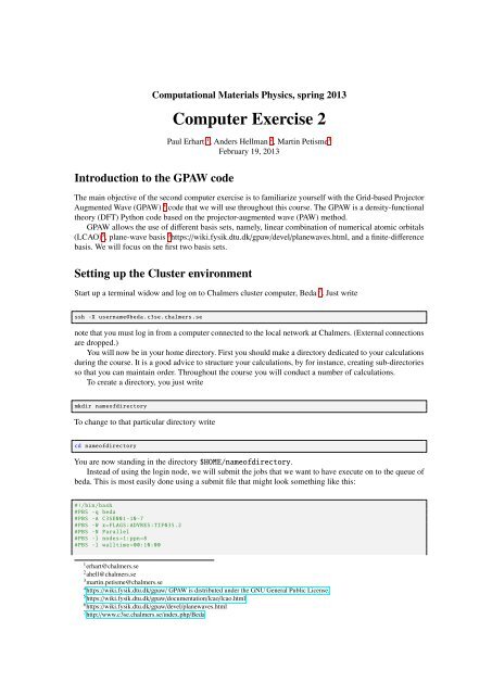
Computational Materials Physics, spring 2013 

Computer Exercise 2 

Paul Erhart 1 , Anders Hellman 2 , Martin Petisme 3 

February 19, 2013 

Introduction to the GPAW code 

The main objective of the second computer exercise is to familiarize yourself with the Grid-based Projector 

Augmented Wave (GPAW) 4 code that we will use throughout this course. The GPAW is a density-functional 

theory (DFT) Python code based on the projector-augmented wave (PAW) method. 

GPAW allows the use of different basis sets, namely, linear combination of numerical atomic orbitals 

(LCAO) 5 , plane-wave basis 6 https://wiki.fysik.dtu.dk/gpaw/devel/planewaves.html, and a finite-difference 

basis. We will focus on the first two basis sets. 

Setting up the Cluster environment 

Start up a terminal widow and log on to Chalmers cluster computer, Beda 7 . Just write 

ssh -X username@beda.c3se.chalmers.se 

note that you must log in from a computer connected to the local network at Chalmers. (External connections 

are dropped.) 

You will now be in your home directory. First you should make a directory dedicated to your calculations 

during the course. It is a good advice to structure your calculations, by for instance, creating sub-directories 

so that you can maintain order. Throughout the course you will conduct a number of calculations. 

To create a directory, you just write 

mkdir nameofdirectory 

To change to that particular directory write 

cd nameofdirectory 

You are now standing in the directory $HOME/nameofdirectory. 

Instead of using the login node, we will submit the jobs that we want to have execute on to the queue of 

beda. This is most easily done using a submit file that might look something like this: 

#!/bin/bash 

#PBS -q beda 

#PBS -A C3SE001 -10-7 

#PBS -W x=FLAGS:ADVRES:TIF035.2 

#PBS -N Parallel 

#PBS -l nodes=1:ppn=8 

#PBS -l walltime =00:10:00 

1 erhart@chalmers.se 

2 ahell@chalmers.se 

3 martin.petisme@chalmers.se 

4 https://wiki.fysik.dtu.dk/gpaw/ GPAW is distributed under the GNU General Public License. 

5 https://wiki.fysik.dtu.dk/gpaw/documentation/lcao/lcao.html 

6 https://wiki.fysik.dtu.dk/gpaw/devel/planewaves.html 

7 http://www.c3se.chalmers.se/index.php/Beda

cd $PBS_O_WORKDIR 

module load COURSES/TIF035 

export GPAW_SETUP_PATH=$PBS_O_WORKDIR:$GPAW_SETUP_PATH 

python ./yourscript.py 

Send the submit file on to the queue by writing 

qsub whateverthenameofthesubmitfile 

Setting up the simulation environment 

First you should load some necessary modules. Type in your terminal 

module load COURSES/TIF035 

Now you are ready to start up ase. However, in this exercise much of you calculations will be conducted 

on the nodes of beda. Hence, you should prepare python-scripts that contain all the information of the 

first-principles calculation you want to do. Use decent editor to write your python scripts, eg. nano, vim, 

Emacs or for a more user-friendly interface use gedit. 

Now it will by much more convenient to write executable script that you can submit through the 

submit-file. Let us use the methane example that you used in exercise 1. 

#!/usr/bin/env python 

from ase import * 

from ase.optimize import BFGS 

from ase.structure import molecule 

import numpy as np 

from gpaw import GPAW 

mol = molecule('CH4') 

mol.center(vacuum=5) 

calc=GPAW(mode='lcao', basis='dzp', h=0.2, xc='PBE', nbands=8, txt='out_task1.txt') 

mol.set_calculator(calc) 

dyn = BFGS(mol , trajectory='mol_task1.traj',logfile='bfgs_task1.log') 

dyn.run(fmax =0.001) 

The difference is the type of calculator used. Now you are calling for GPAW. As the DFT calculator is 

much more complex than the normal potential codes a number of parameters need to be set before one can 

use the GPAW calculator 8 . 

In this case the parameters to the calculator contains the ’mode’, which informs the calculator to use 

linear combination of atomic orbitals (lcao). The ’basis’ tells the calculator to use a double-z function in 

combination with a p-polarization function. This is normally a sufficient basis for the calculations. You 

also provide the flavor of the exchange-correlation functional, i.e, ’xc=PBE’ and the ’h’, which relates how 

accurate the representation of charge density and wavefunctions should be. The arguments ’nbands’ and ’txt’ 

sets the number of KS-orbitals in the simulation and the name of the outputfile, respectively. 

Note that the ’nbands’ needs to be at least as large as the number of electrons in the atomic system. 

Investigate your results by, for instance, using the gui tool included in ase. Open another terminal (you 

need to load the software modules as above) and change to the same directory, than enter the following: 

!ag mol_task1.traj 

8 https://wiki.fysik.dtu.dk/gpaw/documentation/documentation.html 

2

Task 1 

Measure the C–H distance and the H–C–H angle: 

• C–H distance= 

• H–C–H angle= 

Angstrom 

◦ 

How well does the calculator (with a specific basis) do compared to experiment? 

• C–H distance = 1.087 Angstrom 

• H–C–H angle = 109.5 ◦ 

Now let us test the quality of the different basis sets. To do this we will need to generate the basis that 

we should test. GPAW provides a simple tool that allow us to do this. For instance, we are interested in 

generating new basis for hydrogen and carbon only. Type in your terminal 

gpaw -basis -t spz H C 

This will generate a spz bas for each elements. The description of the bas will end up in the library in which 

you created them. This is the reason for the extra line in your submitionfile ’export xxx’, because now GPAW 

to know were to look for the new basis. 

It is important to note that the generation of different basis is a research field in itself, hence, there 

are a number of difficulties that we are skipping over in this course. 

Write a script that tests how well methane properties such as bond distance and angles are calculated 

using the single ζ basis, double ζ basis, triple ζ basis and the same basis sets with a polarization function. 





from ase.parallel import rank 





basisset=['sz','dz','tz','szp','dzp','tzp'] 

for bas in basisset: 

calc=GPAW(mode='lcao', basis=bas , h=0.2, xc='PBE', nbands=8, txt='out.txt') 


dyn = BFGS(mol , trajectory='mol.'+str(bas)+'.traj',logfile='bfgs.log') 

dyn.run(fmax=0.001) 

# Measure O-H distance and H-O-H angle: 

pC = mol.get_positions()[0] 

pH1 = mol.get_positions()[1] 

pH2 = mol.get_positions()[2] 

angle = np.arccos(np.dot(pH1 - pC, pH2 -pC) / 

(np.linalg.norm(pH1 -pC)*np.linalg.norm(pH2 -pC)))*180.0/np.pi 

if rank == 0: 

print 

print 'Current basis set:', bas 

print '--------------------' 

print 'C-H Distance: ', np.linalg.norm(pH1 - pC), 'Angstrom' 

print 'C-H Distance: ', np.linalg.norm(pH2 - pC), 'Angstrom' 

print 'H-C-H Angle: ', angle , 'Degrees' 

3

If you now look inside the output file (’std.out’) it will contain structural information about the water 

molecule and their dependence on the basis functions that you have used in the calculation. 

It could also be good to have an estimate on how much CPU time each basis set contributes with. For 

this kind of test, the water molecule is to small a system. Instead we recall our favorite buckyball, namely 

the C60. 





from ase.data.extra_molecules import data 




import time 

basisset=['sz','dz','tz','szp','dzp','tzp'] 

for bas in basisset: 

atoms = molecule('C60',data=data) 

atoms.center(vacuum=5) 

starttime = time.time() 

calc=GPAW(mode='lcao', basis=bas , h=0.2, xc='PBE', nbands=150, txt='out.txt') 

atoms.set_calculator(calc) 

atoms.get_potential_energy() 

endtime = time.time() 

walltime = endtime - starttime 

if rank == 0: 

print 'Current basis set:', bas 

print '--------------------' 

print 'Wall time:', walltime 

The Molecular Vibration Module 

As a further test of the accuracy of GPAW calculator, let us return to the vibrations of methane. Write a 

script using your favorite basis-set and than calculate the vibrational spectrum of methane. 








from ase.vibrations import Vibrations 





dyn = BFGS(mol , trajectory='mol_task5.traj',logfile='bfgs_task5.log') 


vib = Vibrations(mol) 

vib.run() 

if rank == 0: 

vib.summary() 

for n in range(0,len(mol)*3): 

vib.write_mode(n) 

4

The last line writes out the normal mode into a trajectory file that you can view using the tool ag, by 

writing 

!ag vib.14.traj 

Now you can see and determine which modes are antisymmetric, symmetric, and bending modes by going 

through the different trajectory-files (change the number). 

Task 2 

How is the comparison with experiment? Check on, for instance, the NIST chemistry webbook. 

• Degenerate stretch = 3019 cm −1 

• Symmetric stretch = 2917 cm −1 

• Degenerate deformation mode = 1534 cm −1 

• Degenerate deformation mode = 1306 cm −1 

Try to use your experience of the quality of the basis set to improve the comparison between calculations 

of the vibrational spectra and measurements. What basis set did you use and how did the new vibrational 

modes compare to experiment (look in output.txt)? 

• Basis set = 

• Degenerate stretch = 

• Symmetric stretch = 

• Degenerate deformation mode = 

• Degenerate deformation mode = 

Molecular structure of hydrocarbons 

Let us now repeat the same calculations as above but for the ethane molecule. We basically only change 

’CH4’ to ’C2H6’ in the scripts: 








atoms = molecule('C2H6') 

atoms.center(vacuum=5) 



dyn = BFGS(atoms , trajectory='C2H6.traj', logfile='bfgs_task5.log') 


You will next be asked to calculate the conformational energy in ethane. This you do by rotating the 

hydrogen atoms on one side of the ethane molecule and calculate the energy required for that process. Inside 

the script we also write out the eigenvalues for each rotation into the textfile ”. 

5



from ase.io import read 


from ase.io import PickleTrajectory 



atoms = read('C2H6.traj') 



traj= PickleTrajectory('EthaneRotation.traj', 'w') # makes a trajectory file 

f = open('eigenvalues.txt','w') # Open a file for writing 

f.write('# angle eigenvalue1 eigenvalue 2 ...\n') 

maxstep=60 

for nsteps in range(maxstep): 

newatoms=atoms 

atoms2rot=atoms[2:5] #These are the H atoms that are supposed to be rotated 

angle=2*np.pi/(maxstep) 

rotvector = atoms[0]. position - atoms[1]. position 

atoms2rot.rotate(rotvector ,angle ,center='COM') #This rotates with angle around 

#the z-axis and the center of mass 

pos=atoms2rot.get_positions() 

for n in range(len(atoms2rot)): 

newatoms[n+2]. set_position(pos[n]) 

newatoms.set_calculator(calc) 

traj.write(newatoms) 

eigenvalues = calc.get_eigenvalues() 

eigenvalues_s = ' '.join([str(i) for i in eigenvalues]) 

angle_s = str(angle*(nsteps+1)*180/np.pi) 

# Write angle and eigenvalues to file 

f.write(angle_s + ' ' + eigenvalues_s + '\n') 

f.close() # close file 

Task 3 

Use the ag to look at the trajectory file. How much energy is required to rotate the ethane molecule? The 

experimental value of the barrier is 0.13 eV. 

To understand where the change in the conformational energy comes from we can plot the eigenvalues 

of the KS-system during the rotation. Here we use a script that plots the stored eigenvalues as a function of 

rotation. This you should not send to the queue, but instead run on the login node. 



import pylab as plt 

data = np.loadtxt('eigenvalues.txt') 

angles = data[:,0] 

eigenvalues = data[:,1:] 

plt.plot(angles , eigenvalues , 'o-') 

plt.xlabel('Angle/[degrees]') 

plt.ylabel('K-S eigenvalues/[eV]') 

plt.show() 

How large is the change in eigenvalues (especially the HOMO level)? Given how the total energy is 

evaluated in normal DFT codes (see lecture notes) the conformational energy comes from the change in 

eigenvalues. 

6

1 Home assignment 

As a home assignment you will be asked to calculate the ground state structure of C 2 H 4 . You should try 

to calculate the conformational energy for ethylene. Your results for the conformational energy should 

be analyzed with respect to your knowledge of the molecular orbitals (TIPS: Read about sp3 and sp2 

hybridization). You should include a comparison with C 2 H 6 . 

Note that you will need to modify the script for C 2 H 6 in order to use it for the Home Assignment. 

Furthermore, the task will most probably get you into trouble along the way. Your task is to figure 

out why there is a problem with the script and how to circumvent the problem. It is the 

understanding of the problem (why it happens) that is most important. 

You are suppose to write a report about your first-principles investigation. Needless to say it should be 

well written and nicely presented. 

• Abstract (Present the task and give the main results. This part should be self-explained) 

• Introduction (Give some background and than try to explain the task and how you aim to solve it) 

• Computational method (code, calculator parameters, size of cell, elements, length of simulation and 

other relevant criteria) 

• Results (figures showing energies, perhaps figures showing the snapshots of trajectories, text that 

descries the results in a qualitative manner) 

• Discussion (Try to bring order in your results, rationalize the results to the best of your ability) 

• Conclusions 

• Appendix (Add your script(s) that you have used to solve the task) 

Remember that the report will be graded! Deadline is Tuesday 26/2 at 12:00. 

7

Computer Exercise 2 - Fysik

Create successful ePaper yourself

Delete template?

Save as template?