The Projector Augmented Wave method
The Projector Augmented Wave method
The Projector Augmented Wave method

Create successful ePaper yourself
Turn your PDF publications into a flip-book with our unique Google optimized e-Paper software.
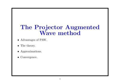
<strong>The</strong> <strong>Projector</strong> <strong>Augmented</strong><strong>Wave</strong> <strong>method</strong>• Advantages of PAW.• <strong>The</strong> theory.• Approximations.• Convergence.1
<strong>The</strong> PAW <strong>method</strong> is ...What is PAW?• A technique for doing DFT calculations efficiently and accurately.• An all-electron <strong>method</strong> with easy-to-control approximations.• An elegant theory.• A <strong>method</strong> that works with smooth pseudo wave-functions thatcan be expanded in a few plane waves (or expressed on coarsegrids).• Ultra-soft pseudopotentials done right!2
Literature<strong>The</strong> PAW <strong>method</strong> was invented by Peter Blöchl in 1994:• ”<strong>Projector</strong> augmented-wave <strong>method</strong>”, P. E. Blöchl, Phys. Rev. B50, 17953 (1994)• ”<strong>Projector</strong> augmented wave <strong>method</strong>: ab initio moleculardynamics with full wave functions”, P. E. Blöchl, C. J. Först andJ. Schimpl, Bull. Mater. Sci, 26, 33 (2003)• ”Real-space grid implementation of the projector augmentedwave <strong>method</strong>”, J. J. Mortensen, L. B. Hansen, and K. W.Jacobsen, Phys. Rev. B, 71 035109 (2005)3
Advantages of PAW• No need to deal with inert core electrons.• Valence pseudo wave functions are smooth and without nodesinside the augmentation spheres.• Access to full all-electron wave functions and density. Useful fororbital-dependent XC-functionals.4
Platinum atom43211s2s3s4s5s6s2p3p4p5p3d4d5d0-1-20 1 2 3 4r (Bohr)5
Augmentation SpheresOne cutoff radius for each type of atom. Spheres should not overlap:6
Electron densityn= ñ plane waves/coarse grid+ ∑ a na logarithmic radial grids− ∑ a ñalogarithmic radial grids7
<strong>The</strong> PAW transformationψ n (⃗r) = ˆτ ˜ψ n (⃗r)ˆτ = 1 + ∑ a∑(|φ a i 〉 − | ˜φ a i 〉)〈˜p a i |,iwhere ˜p a i (⃗r) = 0 and ˜φ a i (⃗r) = φa i (⃗r) for r > ra c , and 〈˜p a i | ˜φ a j 〉 = δ ij.|˜p a i 〉 = ˜p a nlm(⃗r − ⃗R a ) = ˜p a nl(r)Y lm ( ⃗r − ̂ ⃗R a )ˆτ ˜φ a i = φ a i8
Completeness relationsFor |⃗r − ⃗R a | < rc a we must have:∑| ˜φ a i 〉〈˜p a i | = 1iFrom this follows that inside the augmentation spheres, ψ n and ˜ψ ncan be expanded in partial waves and pseudo partial wavesrespectively:| ˜ψ n 〉 = ∑ i| ˜φ a i 〉〈˜p a i | ˜ψ n 〉.|ψ n 〉 = ∑ i|φ a i 〉〈˜p a i | ˜ψ n 〉,In the interstitial region, we have ψ n = ˜ψ n .9
Electron density (again)n(⃗r) = ∑ an a c (|⃗r − ⃗R a |) + ∑ nf n |ψ n (⃗r)| 2= ∑ an a c + ∑ nf n∣ ∣∣∣∣˜ψn + ∑ ai〈˜p a i | ˜ψ n 〉(φ a i − ˜φ a i )∣2= ∑ n a c + ∑ f n | ˜ψ n | 2a n+ ∑ ∑f n 〈˜p a i | ˜ψ n 〉(φ a i − ˜φ a i )〈 ˜ψ n |˜p a j 〉(φ a j − ˜φ a j )n aij⎧⎫⎪⎨ ∑ ∑ ∑+2Re f n 〈˜p a i |⎪⎩˜ψ n 〉 ˜φ∑⎪⎬ai 〈 ˜ψ n |˜p a j 〉(φ a j − ˜φ a j )n a ij⎪⎭} {{ }˜ψ n10
Electron density (continued)n = ∑ nf n | ˜ψ n | 2 + ∑ aijD a ij(φ a i φ a j − ˜φ a i ˜φ a j ) + ∑ an a c ,where we have defined atomic density matrices as:D a ij = ∑ n〈˜p a i | ˜ψ n 〉f n 〈 ˜ψ n |˜p a j 〉11
Electron density (continued)With these definitions:n a = ∑ ijD a ijφ a i φ a j + n a c ,ñ a = ∑ ijD a ij ˜φ a i ˜φ a j + ñ a c ,ñ = ∑ nf n | ˜ψ n | 2 + ∑ añ a c ,we get a very simple expression for the all-electron density:n = ñ + ∑ a(n a − ñ a )12
Compensation chargesLet Z a (⃗r) be the nuclear charge for atom a. <strong>The</strong> Coulomb energy is:(∫ n(⃗r) + ∑ ) (E C = d⃗rd⃗r ′ a Za (⃗r − ⃗R a ) n(⃗r ′ ) + ∑ )a Za (⃗r ′ − ⃗R a )|⃗r − ⃗r ′ |= (n + ∑ aZ a ) 2= (ñ + ∑ a[n a − ñ a + Z a ]) 2We add and subtract compensation charges localized inside theaugmentation spheres:E C = (ñ + ∑ a˜Z a + ∑ a[n a − ñ a + Z a − ˜Z a ]) 213
Compensation charges (continued)<strong>The</strong> compensation charges are constructed like this:˜Z a (⃗r) = ∑ lmQ a lm˜g a lm(⃗r),where ˜g a lm (⃗r) = 0 for r > ra c :˜g a lm(⃗r) = C l r l exp(−α a r 2 )Y lm (ˆr),<strong>The</strong> Q a lm ’s are chosen such that na − ñ a + Z a − ˜Z a has no multipolemoments: ∫d⃗rr l Y lm (ˆr)(n a − ñ a + Z a − ˜Z a ) = 014
Compensation charges (continued)Using ˜ρ = ñ + ∑ a ˜Z a , ˜ρ a = ñ a + ˜Z a and ρ a = n a + Z a , we get:E C = (ñ + ∑ a˜Z a + ∑ a[n a − ñ a + Z a − ˜Z a ]) 2= (˜ρ + ∑ a[ρ a − ˜ρ a ]) 2= ˜ρ 2 + 2˜ρ ∑ a(ρ a − ˜ρ a ) + ∑ ab(ρ a − ˜ρ a )(ρ b − ˜ρ b )Since ρ a − ˜ρ a has no multipole moments, we get:E C = ˜ρ 2 + 2 ∑ a˜ρ a (ρ a − ˜ρ a ) + ∑ a(ρ a − ˜ρ a ) 2= ˜ρ 2 + ∑ a(ρ a ) 2 − ∑ a(˜ρ a ) 2 (1)15
Finally ...... we have E C = ẼC + ∑ a (Ea C − Ẽa C ), where ẼC has contributionsfrom all of space:(∫ ñ(⃗r) + ∑ ˜ZẼ C = d⃗rd⃗r ′ a a (⃗r − R ⃗ ) (a ) ñ(⃗r ′ ) + ∑ ˜Z a a (⃗r ′ − R ⃗ )a )|⃗r − ⃗r ′ ,|and EC a − Ẽa C is a correction from each augmentation sphere:()∫EC a = d⃗rd⃗r ′ (na (⃗r) + Z a (⃗r)) n a (⃗r ′ ) + Z a (⃗r ′ )|⃗r − ⃗r ′ ,|(∫ ñ a (⃗r) + ˜Z) ()a (⃗r) ñ a (⃗r ′ ) + Z a (⃗r ′ )ẼC a = d⃗rd⃗r ′ |⃗r − ⃗r ′ |16
• Frozen core states.Approximations• Truncated multipole expansion of compensation charges.• Finite number of projectors, partial waves and pseudo partialwaves:– Hydrogen: 2 s-type, 1 p-type.– Oxygen: 2 s-type, 2 p-type, 1 d-type.– Copper: 2 s-type, 2 p-type, 2 d-type.• Overlapping augmentation spheres:17
Kinetic energyE kin = Ẽkin + ∑ a(E a kin − Ẽa kin),whereẼ kin = − 1 2∑∫f nd⃗r ˜ψ ∗ n∇ 2 ˜ψn∑∫n∑core∫E a kin = − 1 2D a ijd⃗rφ a i ∇ 2 φ a j − 1 2d⃗rφ a c∇ 2 φ a cijẼ a kin = − 1 2∑∫cD a ijd⃗r ˜φ a i ∇ 2 ˜φa jij18
Exchange-correlation energyE xc = Ẽxc + ∑ a(E a xc − Ẽa xc),where∫Ẽ xc = d⃗rñɛ xc [ñ]∫Exc a = d⃗rn a ɛ xc [n a ]∫Ẽxc a = d⃗rñ a ɛ xc [ñ a ]19
HamiltonianE = Ẽ + ∑ ∆E a (D a δEij),aδ ˜ψ= f n Ĥ ˜ψ nn∗Ĥ = − 1 2 ∇2 + ṽ + ∑ ∑|˜p a i 〉∆Hij〈˜p a a j |,aijwhere ṽ = δẼ/δñ = ṽ H + ṽ xc and∆H a ij = ∆Ea∂D a ij+ ∑ lm∂Q a lm∂D a ij∫d⃗rṽ H˜g a lm<strong>The</strong> PAW <strong>method</strong> is a generalized Kleinman-Bylander nonlocalpseudopotential that adapts to the current environment!20
OrthogonalityKeep the wave functions orthogonal:δ nm = 〈ψ n |ψ m 〉 = 〈 ˜ψ n |Ô| ˜ψ m 〉,whereandÔ = 1 + ∑ a∆O a ij =∫∑|˜p a i 〉∆Oij〈˜p a a j |ijd⃗r(φ a i φ a j − ˜φ a i ˜φ a j )21
PBE atomization energy of anitrogen moleculefrom ASE import Atom , ListOfAtomsfrom gridpaw import Calculatora = 8.0 # size of unit cellh = 0.18 # grid spacingN = ListOfAtoms ([ Atom (’N’ , (0 , 0 , 0) , magmom =3)],cell =(a , a , a) , periodic =1)calc = Calculator ( nbands =4 , xc=’PBE ’ , h=h)N. SetCalculator ( calc )e1 = N. GetPotentialEnergy()d = 1.1 # bond lengthN2 = ListOfAtoms ([ Atom (’N’ , [0 , 0 , 0]) ,Atom (’N’ , [0 , 0 , 1.1]) ],cell =(a , a , a) , periodic =1)calc = Calculator ( nbands =5 , xc=’PBE ’ , h=h)N2. SetCalculator ( calc )e2 = N2 . GetPotentialEnergy()print 2 * e1 - e2 , ’eV ’22
Convergencespd 11 22 221 222 321 231∆E (eV) 10.016 10.141 10.520 10.519 10.519 10.514l max 0 1 2∆E (eV) 10.520 10.574 10.560Dacapo Blaha et al. Experiment∆E (eV) 9.611 10.546 9.90923