

Analysis of Spatial Dynamic Correlation and Influencing Factors of Atmospheric Pollution in Urban Agglomeration in China
1
School of Economics and Management, Hefei Normal University, Hefei 230601, China
2
School of Accounting, Anhui University of Finance and Economics, Bengbu 233030, China
3
School of Management, University of Science and Technology of China, Hefei 230026, China
*
Author to whom correspondence should be addressed.
Sustainability 2022, 14(18), 11496; https://doi.org/10.3390/su141811496
Submission received: 11 August 2022
/
Revised: 8 September 2022
/
Accepted: 9 September 2022
/
Published: 14 September 2022
(This article belongs to the Collection Air Pollution Control and Sustainable Development)
Abstract
:The fluidity of air pollution makes a cross-regional joint effort to control pollution inevitable. Exploring the dynamic correlation and affecting factors of air pollution in urban agglomerations is conducive to improving the effectiveness of pollution control and promoting the high-quality development of the regional economy. Based on daily data on PM2.5 concentration, the article identifies the dynamic association relationship of atmospheric pollution in urban agglomerations of Beijing–Tianjin–Hebei (BTH) air pollution transmission channel under the framework of the vector autoregressive model, building the spatial correlation network of atmospheric pollution in urban agglomerations of BTH atmospheric pollution transmission channel, investigating the structure characteristics and influencing factors. The results show that the atmospheric pollution in BTH cities has a general dynamic correlation, which shows a stable multithreaded complex network structure; the overflow direction of air pollution is highly consistent with the weight matrix of northwest wind direction; economic development level, population density, openness degree, geographical location, and the relationship of wind direction are the important factors affecting the spatial association network of atmospheric pollution. We should actively explore the construction mode of urban agglomeration under the constraint of atmospheric pollution and improve the cross-regional collaborative governance mechanism.
1. Introduction
Given the early extensive economic growth model, inefficient energy use efficiency, the high proportion of coal, and, in the end, energy consumption, atmospheric pollution has wreaked havoc in many Chinese cities since 2012. The pattern of urban expansion characterized by high-density construction and high-intensity consumption of resources further leads to more frequent and wider outbreaks of urban air pollution in China. Chinese people should work together to control air pollution, and air quality in Chinese cities has improved markedly. The 2020 World Air Quality Report showed that 86 percent of Chinese cities had higher air quality than the previous year, and the PM2.5 exposure levels of the population had dropped by 11 percent. However, China still dominates the list of the 100 most polluted cities in the world, despite continuous improvements in urban air quality. According to the 2020 China Environmental Bulletin, air quality in 135 out of 337 cities exceeded the standard, with PM2.5 being the main culprit among pollutants.
The atmosphere is fluid, and air pollution has the characteristics of spatial agglomeration and diffusion [1,2,3,4]. Each 1% increase in the Air Quality Index of neighboring cities will lead to a 0.45% increase in the Air Quality Index of the city [5]. Spatial spillover effect and regional agglomeration features of atmospheric pollution mean “unilateral” efforts to treat haze may become in vain because of the regional haze pollution “leakage effect” [6]. In view of the spread of air pollution, any individual industrial structure adjustment in any region is ineffective. Only by coordinating with each other and establishing a joint prevention and control mechanism can achieve the goal of coordinated air pollution control [7].
Atmospheric pollution will reduce the attractiveness of cities and thus slow down the process of urbanization [8]. First of all, atmospheric pollution has a significant effect on the healthy life of urban people. Long exposure to a bad air environment will increase respiratory infections, cardiovascular and cerebrovascular diseases, and even cause premature death, increasing health costs [9,10]. Secondly, with the expansion of cities, the weight of the ecological environment in population competitiveness is increasing, and urban air pollution may lead to a decrease in the floating population’s residence intention, resulting in the “reverse urbanization” phenomenon, hindering the promotion of new urbanization strategy and having a negative impact on urban development [11]. Some scholars think that the decline of air quality in big cities is an important factor restricting labor supply, resulting in the “expelling effect” of human capital [12], and groups with high human capital are more sensitive to the air pollution [13].
The BTH region is located in eastern China, where the northwest wind prevails and in the semi-closed terrain of Taihang Mountain and Yanshan Mountain. Pollutants are easy to accumulate there, and the region has a high level of urbanization and a high population density [14]. In addition, coal is the main source of energy, and environmental governance problems have been prominent. As the air pollution transmission channel of The BTH region, the urban agglomeration is an essential part of China’s core economic zone, with a high proportion of GDP. However, the contradiction between economy and environment is prominent. The Ecological and Environmental Conditions report of China in 2020 shows that 15 cities in the urban agglomeration of BTH atmospheric pollution transmission channel, including Anyang, Shijiazhuang, and Taiyuan, were ranked in the bottom 20 among 168 cities in the urban ambient air quality comprehensive index in 2020; the average number of good days in the urban agglomeration was 63.5%, much lower than the 87.0% average; the average PM2.5 concentration in 2020 was 51 micrograms per cubic meter, much higher than the average concentration in the Yangtze River Delta, another key region (35 micrograms per cubic meter).
Air pollution control is complicated by the transport of air pollutants in neighboring areas; the BTH region is also facing the double pressure of improving regional air quality and controlling cross-regional pollution. It is urgent to explore the regional atmospheric pollution dynamic association of space and its influence factors, to search for ways to establish trans-regional coordinated prevention and control of air pollution, to win the battle of pollution prevention and governance, to promote coordinated development between regions, to boost the joint law enforcement action to improve air quality improvement effect. Spatial autocorrelation analysis originated from biometrics and has become one of the basic methods in theoretical geography [15]. Spatial data are almost all spatially dependent, so the study of regional pollution coordination and governance is no exception. Exploratory spatial data analysis has been used in several pieces of literature to analyze the spatio-temporal characteristics and interactive effects of regional air quality in China [16,17,18,19]; The existing literature on air pollution in the process of urban expansion is mostly based on static analysis and lacks dynamic excavation of the spatial-temporal evolution of internal air pollution within urban agglomerations. The spatial weight is mainly set by the spatial geographic weight matrix or spatial adjacent weight matrix [16,20,21]. However, the vector wind has a certain ability to explain the variation of PM2.5 concentration [22]. The prevailing monsoon transported PM2.5 from the upwind region to the downwind region; PM2.5 concentration is generally affected by wind direction [23]. The east of China is a monsoon region, and the northwest wind prevails in autumn and winter in the “2 + 26” urban agglomeration. the northwest wind is essential in the diffusion of PM2.5. Therefore, attention should be paid to the new characteristics of spatial spillover of urban agglomeration.
The marginal contribution of this paper lies in: First, in terms of the selection of research regions, the BTH region and its surrounding areas, which are called the BTH air pollution transmission channel urban agglomeration, are selected as the research object to highlight the air quality changes of urban agglomeration and the correlation between surrounding cities. This area is one of the typical key pollution regions and has better representativeness in China. Second, based on daily PM2.5 data, to analyze the spatial dynamic correlation structure characteristics between urban agglomerations in typical regions and thoroughly and meticulously sort out the dynamic correlation relationship between cities, which can provide new empirical evidence for the joint prevention and control of air pollution in other key regions. Third, taking into full account the fact that the strong northwest wind in autumn and winter caused long-term air pollution in the urban agglomeration of the BTH atmospheric pollution transmission channel, the spatial weight matrix of wind direction was constructed, presenting a new feature of the spatial spillover direction of air pollution.
The remainder of the paper is arranged as follows: Section 2 is the research model and data description of the spatial dynamic correlation of air pollution in the urban agglomeration of the BTH air pollution transmission channel. Section 3 presents the empirical results and analysis. Section 4 summarizes the conclusion and offers proposals.
2. Model and Data
2.1. Model Construction
2.1.1. Spatial Correlation Analysis
In order to explore whether air pollution has the characteristics of non-randomness and spillover effect in spatial distribution, the exploratory spatial analysis method was used, and Moran’s Index was adopted to investigate the overall spatial distribution characteristics of PM2.5. The formula is as follows [24]:
where is the total city number in the research sample; and , respectively, represent the observed value of PM2.5 of city and city ; presents the average value of PM2.5; and is the spatial weight matrix.
Three matrices are respectively selected in this paper. The first is the weight matrix of spatial wind direction (), which presents the transmission effect of northwest wind on PM2.5 diffusion in the urban agglomeration of the BTH air pollution transmission channel, measuring the spatial dynamic correlation of air pollution taking a city as a unit. If the northwest wind of the city comes from the upwind city , the value is 1; otherwise, the value is 0. The second is the spatial adjacent weight matrix (). If the city and city is adjacent, the value is 1; otherwise, it is 0. The third is the geographical distance weight matrix (); according to the first law of geography, the longer the distance between two places, the weaker the spatial connection effect will be; therefore, the reciprocal of geographical distance is used to construct geographical distance weight matrix [25].
The Moran’s value is between −1 and 1. If the value approaches 0, there is no spatial autocorrelation of air pollution. If it is greater than 0, air pollution has a positive spatial correlation, indicating the areas with similar air pollution concentrations are clustered together. If it is less than 0, air pollution is negatively correlated in space, indicating that areas with different concentrations of air pollution are clustered together.
2.1.2. Spatial Network Correlation Measurement of Air Pollution
The social network analysis method is a kind of interdisciplinary analysis method aiming at “relational data” and taking “relationship” as the basic analysis unit. It builds the association network and carries out global analysis and structural relationship analysis. In this paper, the spatial correlation network is the relational set of air pollution of each city in the BTH air pollution transmission channel urban agglomeration. Each city is a point in the network, and the air pollution correlation relationship between cities are lines in the network. The network composed of points and lines can clearly reflect the spatial dynamic correlation of air pollution in urban agglomeration along the air pollution transmission channel.
In this paper, the method of Granger causality test was used to identify spatial associations and correlations of the urban agglomerations. Based on the unit root stationarity test of PM2.5 concentration series in 28 cities, the function model of PM2.5 concentration series variables between two cities in 28 cities was established, namely the vector autoregression model (VAR) [21].
where and are the time series variables of the air pollution level of any two cities; , , , and are the lags; , , , , , and are parameters to be estimated; and are random disturbance terms. The Granger causality test is conducted under the framework of the VAR model above-mentioned, and the significance level of 5% is taken to determine the spatial correlation. If is significant at 5% significance level, it is considered that the atmospheric pollution concentration of city can be explained by the pollution concentration of city , that is, the air pollution of city produces a spillover effect on city , and the corresponding element of the spatial correlation matrix is obtained; otherwise, the value is 0, and the corresponding element of spatial correlation matrix . Similarly, if is significant at 5% significance level, it is considered that the atmospheric pollution concentration of city can be explained by the pollution concentration of city , that is, the air pollution of city has a spillover effect on city , and the value is assigned to 1; otherwise, the value is assigned to 0. There are four possibilities in the test results, that is, one-way correlation, two-way correlation, or no correlation between city and city . Thus, the spatial correlation matrix of air pollution between cities is constructed, which can represent the spatial correlation network system of the urban agglomeration of the BTH air pollution transmission channel.
In the network system, individual characteristics directly reflect the relative importance and status of each city. The characteristics of individual network structure can be characterized by out-degree centrality, in-degree centrality, point centrality, closeness centrality, and betweenness centrality. Out-degree centrality is the relationship number emitted by this node, which represents the spillover influence of one city on other cities in the networks. In-degree centrality is the number of relationships received by this node, which represents the influence that a city receives from other cities on it. The software can automatically calculate the out-degree centrality and in-degree centrality. Point centrality is used to measure the ability of a city to produce a linkage relationship of air pollution with other cities; it is measured by the number of cities directly connected with other cities. The high point centrality of a city shows the city is directly connected with others, and it is in the center of the network. Closeness centrality measures the extent to which a city is not controlled by other cities and reflects the independence of the city in the network; if the “distance” of a city is very short, the city has a high degree of closeness to the center, and the city has a rapid influence on the spatial linkage of air pollution. Betweenness centrality is an index representing “control ability”, which mainly measures how much each city is located in the “middle” of other cities in the network. The higher the betweenness centrality of a city is, the stronger the city’s ability to control the air pollution associations of other cities is.
Equations (4)–(6) are the calculation methods of point centrality, betweenness centrality, and closeness centrality [26].
is the associated number of nodes , and is the network scale.
represents a shortcut between nodes and .
represents the total number of shortcuts that pass-through node between nodes and . , and .
2.1.3. QAP Regression Analysis
Based on Environmental Kuznets Curve theory, taking into account geographical distance, meteorological and socioeconomic factors, the influencing factor model of air pollution spatial association network is constructed as follows:
All variables in model (7) are matrices, where presents the spatial correlation matrix of air pollution in the urban agglomeration, which is obtained from the VAR model above. The geographical distance factor is the spatial adjacency matrix of the urban agglomeration of the BTH air pollution transmission channel; the meteorological factor is the relationship matrix of wind direction between cities. Social and economic factors include economic development (), population density (), industrial structure (), degree of openness (), fiscal freedom (), and energy consumption structure (). is the difference matrix of economic development level between cities and the per capita is used to measure the economic development level of each city. is difference matrix of population density between cities, population density is described by the population number of per unit area of each city. Industrial is the difference matrix of Industrial structure between cities; the industrial structure is measured by the secondary industry proportion of cities. is the difference matrix of openness degree between cities, the actual amount of foreign direct investment used by each city represents the level of openness degree of a city. is the difference matrix of Fiscal freedom between cities, the ratio of budgetary Fiscal revenue and budgetary Fiscal expenditure in each city is selected to measure Fiscal freedom. is the difference matrix of Energy consumption structure between cities. Referring to relevant literature [16], this paper selects the proportion of the output of the high-consumption coal industry in regional as an indicator to measure energy consumption structure.
Model (7) adopts QAP (Quadratic Assignment Process) analysis. The spatial correlation data of urban air pollution belong to relational data, which generally cannot be tested by traditional statistical testing methods because there may be a high degree of correlation between these relational data. QAP is a method based on matrix data replacement, which compares the similarity of each lattice value in the two square matrices, the correlation coefficient between the two matrices is obtained, and the correlation coefficient is tested non-parametrically [27]. The QAP analysis method does not need to assume that the independent variables are independent of each other, which is more robust than the parametric method [28].
2.2. Data Sources
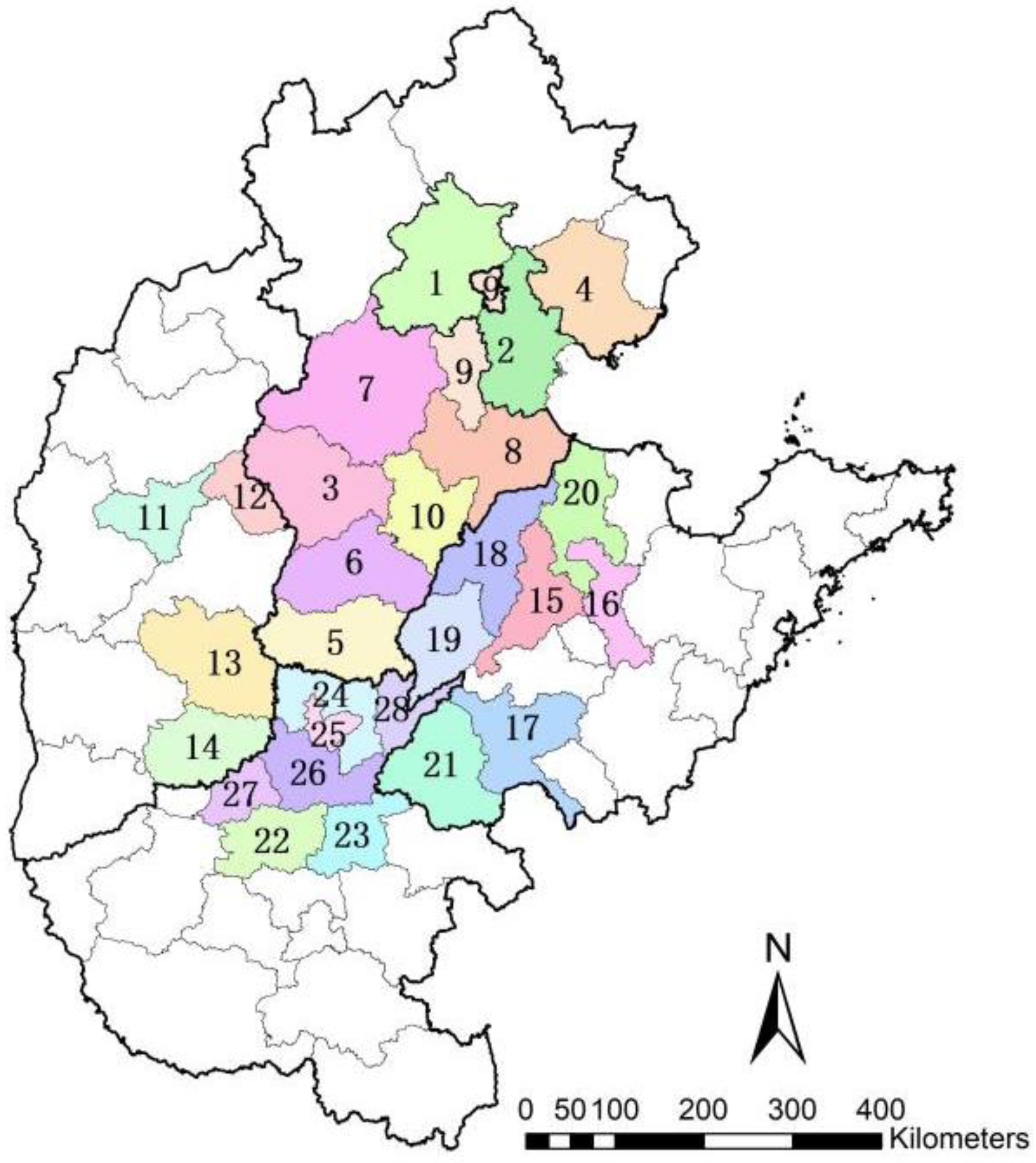
The research object of this paper is the Urban agglomeration of the BTH air pollution transmission channel, which specifically includes 28 cities. The geographical locations of the 28 cities are shown in Figure 1. Although these cities belong to different administrative regions, they are an inseparable whole in terms of air pollution.
PM2.5 concentration is selected to measure the urban air pollution level. Compared with the traditional air pollution index, PM2.5 source and composition are more complex, and the harm degree is higher, which is the “culprit” of pollutants.
The data period in this paper is from 1 January 2020 to 31 December 2021. The daily data of PM2.5 concentration were obtained from the website of “Weather Report” through the web crawler program, the website is www.tianqihoubao.com/aqi (accessed on 1 September 2022). The annual average processing of daily data of PM2.5 concentration was carried out during the spatial correlation analysis. During QAP analysis, the period from 2016 to 2020 was selected as the sample observation period to calculate the average value of the corresponding index in model (7) during the investigation period, and then the absolute difference of the average value constituted the corresponding difference matrix. All data were from statistical yearbooks, statistical gazette, and China Economic Network statistical database of 28 cities over the years.
3. Empirical Results
3.1. Spatial Correlation of Air Pollution in Urban Agglomeration
According to the above Formula (1), the universe spatial correlation index of PM2.5 was calculated, and the results are shown in Table 1. Based on the Moran’s I results in Table 1, the spatial wind direction weight matrix (), spatial adjacent weight matrix (), and spatial inverse geographical distance weight matrix () were selected. At the significance level of 1% or 5%, the universe Moran’s was significantly positive. The results show that air pollution in the urban agglomeration of the BTH atmospheric pollution transmission channel has a significant positive correlation.
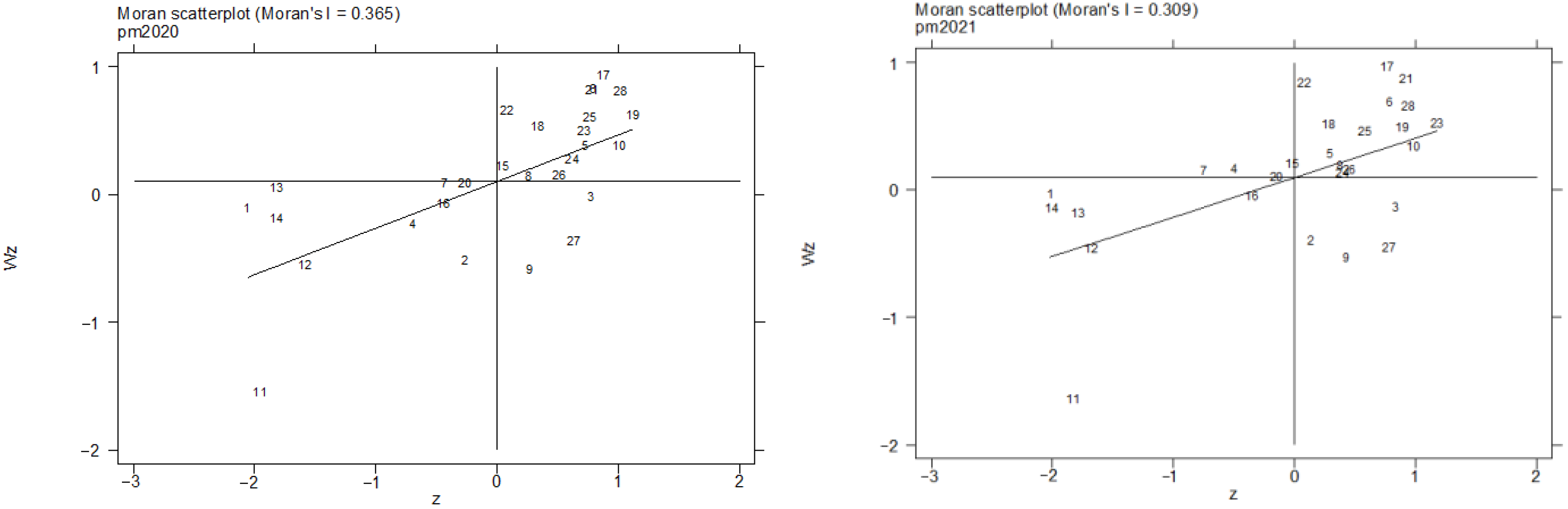
The spatial wind weight matrix () was further selected to draw the Moran scatter diagram, which showed that most cities lay in the first and third quadrants, and only a few lay in the second and fourth quadrants, presenting high–high aggregation mode (H–H) and low–low aggregation mode (L–L). As shown in the Figure 2, there is a positive correlation between the spatial distribution of air pollution.
3.2. Characteristics of Spatial Association Network of Air Pollution in Urban Agglomeration
3.2.1. Overall Network Characteristics
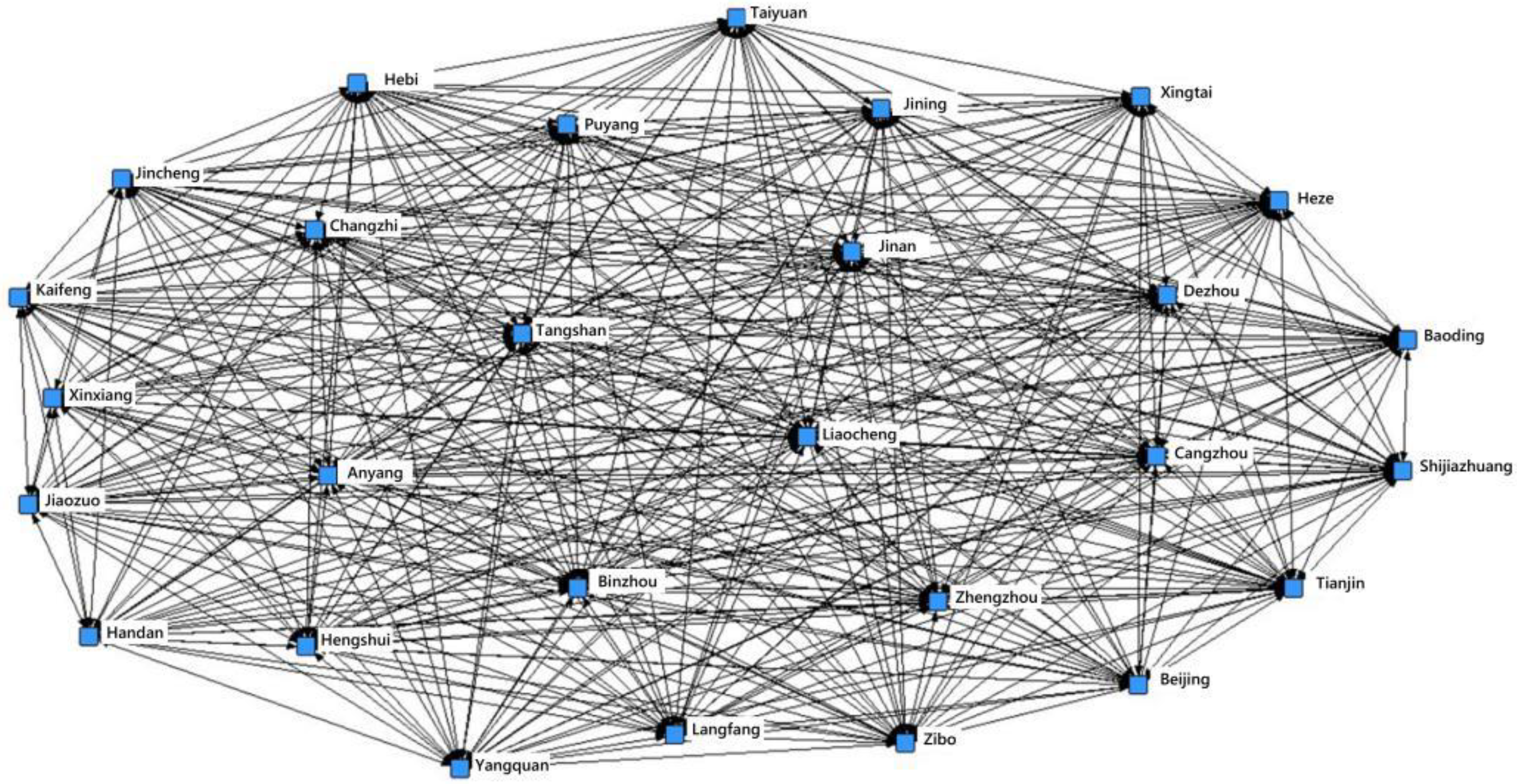
The net-draw tool of UCINET was used for visualizing the processing above, as shown in Figure 3. There is no independent point in the spatial correlation of the network; the PM2.5 concentration of urban agglomeration presents a complex and multithreaded spatial correlation. The air pollution of a city is not only affected by local meteorological and socioeconomic factors but also associated with other atmospheric pollution of the city, and the relationship goes beyond mere geography in the sense of “adjacent” or “similar” effect; each city has at least one more spatial correlation.
The overall network density of the air pollution spatial correlation network is 0.872, indicating that the air pollution of each city in the network has a very close correlation, the air pollution spatial correlation breaks through the pure relationship between adjacent cities and presents a multithreaded cross network distribution; the measurement result of network correlation degree is 1, shows that the 28 cities are all correlated with each other in air pollution, and the accessibility between cities in the network is very high, there is no isolated city, and the network is very robust, and every city is directly affected by the spatial network. Overall speaking, there is a general spatial dynamic correlation between air pollution in various cities. The network has a high degree of accessibility, which belongs to a relatively uniform structure, with decentralized power and low level. Each city can easily generate spatial correlation with other cities, which also indicates that it is difficult for any city to be “isolated” in pollution control.
3.2.2. Individual Network Characteristics
Table 2 shows the node characteristics of the spatial association network during the sample observation period.
As shown in Table 2, the mean values of out-degree centrality and in-degree centrality are both 23.54. Among them, there are 21 cities whose out-degree centrality is over the mean value, indicating the air pollution of these cities will spill out to others and have a great impact on others. There are 18 cities with in-degree centrality greater than the mean, indicating that these cities are more susceptible to air pollution than other cities. The cities with the highest out-degree centrality of 27 are Zhengzhou and Anyang in Henan Province and Shijiazhuang in Hebei Province, indicating that these three cities have the strongest radiation and are most likely to affect the air pollution level of others. Several cities have the highest in-degree centrality of 27, indicating they are in the middle of the air pollution networks and are most susceptible to the impact of air pollution fluctuations of other cities. They are Jinan, Jining, Zibo, Dezhou in Shandong Province, and Cangzhou in Hebei Province.
The mean point centrality of BTH air pollution transmission channel urban agglomeration was 87.170. There are 14 cities above the average, from high to low, Shijiazhuang, Zhengzhou, Dezhou, Changzhi, Kaifeng, Jiaozuo, Hengshui, Puyang, Jincheng, Binzhou, Cangzhou, Taiyuan, Yangquan, and Hebi; there are many correlations between air pollution in these cities and other cities. Among them, five cities belong to Henan Province, four cities belong to Shanxi Province, three cities belong to Hebei Province, and two cities belong to Shandong Province. Therefore, comparatively speaking, Henan province and Shanxi Province are regions with relatively concentrated spatial correlation in air pollution. The three cities with the least number of spatial correlation relationships are Jining, Jinan in Shandong Province, and Beijing; these cities are located at the edge of the network and are less connected to other cities.
According to the closeness centrality, the mean value of the urban agglomeration was 89.810, and 14 cities were higher than the mean value, which were Shijiazhuang, Zhengzhou, Dezhou, Changzhi, Kaifeng, Jiaozuo, Hengshui, Puyang, Jincheng, Binzhou, Cangzhou, Taiyuan, Yangquan, and Hebi in turn. These cities can quickly associate with other cities in the spatial association network and are network centric actors in the network.
As to the betweenness centrality, the top six cities are Taiyuan, Jincheng, and Changzhi in Shanxi Province, Shijiazhuang in Hebei province, and Zhengzhou and Kaifeng in Henan Province. It can be seen that some cities of Shanxi Province and other provincial capitals are relatively in the central position, playing the role of “intermediary” and “bridge”, and have a strong influence on air pollution in other cities.
The measurement results of individual network characteristics show that Shanxi Province and provincial capitals are the most likely to affect the air pollution of other cities, and cities in Shandong Province are the most likely to be affected by other cities, while Beijing is a relatively independent position. The reason is that Shanxi Province is China’s first coal production, coal transport province, and energy-heavy chemical base; coal is its main resource, coal combustion process produces not only a large number of soot but also the formation of carbon monoxide, carbon dioxide, sulfur dioxide, nitrogen oxides, and other harmful substances, aggravating the air pollution of the city. Shandong province is located in the northwest of other cities and is affected by the northwest wind. The air pollutants of Shanxi Province and other cities will be transmitted and diffused to Shandong Province through the northwest wind, aggravating the air pollution of Shandong Province. Therefore, Shandong province is more vulnerable to air pollution from other cities. Beijing is located on the northern edge of the urban cluster. Due to its own unique geographical location and meteorological factors, it is in a relatively “independent” position in the urban agglomeration and has relatively little correlation with the air pollution of other cities.
3.3. Influencing Factors of Spatial Association Network in the Urban Agglomeration
The QAP method was used for regression of model (7), and 5000 random replacements were selected, obtaining the QAP regression results of the spatial correlation matrix and influencing factors of air pollution in the urban agglomeration, as shown in Table 3.
The results of QAP regression show that 5000 random displacement and within the range of sample volume of 756 (the total number of interrelated influences of 28 cities), the adjusted determination coefficient is 0.324, indicating that the variable explanatory power of the regression model to air pollution spatial network association was 32.4%. Among them, the regression coefficient of spatial adjacency matrix is −0.1269, indicating geographical proximity does have an important effect on the spatial correlation of urban agglomeration air pollution, which is consistent with the research conclusion of Lin L and Li J [29]. The regression coefficient of the wind direction relation matrix was −0.2596, indicating the northwest wind would significantly affect the spatial correlation relationship of air pollution, which according to the view of Wang ZJ et al. [30], mentioned that meteorological factors would affect the concentration and diffusion of atmospheric particles, and there are leading, and lagging relations of atmospheric concentration between cities are similar. The coefficient of of the difference matrix of economic development level is negative and close to 0, indicating the difference in economic development level between cities has a significant impact on the spatial correlation of air pollution, but the effect is not obvious. The regression coefficient of the population density difference matrix is positive, indicating the greater the difference in population density between cities, the more air pollution conduction relationship is. Areas with high population density are not conducive to the diffusion of pollutants due to the influence of high residential density on wind speed. Therefore, the greater the difference in population density between cities, the more obvious the diffusion effect of pollutants is. The gap matrix of openness degree between Cities is negative, indicating that the greater the similarity of openness between cities is, the greater the conduction relationship and spatial spillover effect of air pollution between cities are. Compared with community economy factors, geographical location and meteorological factors have a greater direct impact on the spatial correlation of air pollution. While the financial freedom difference matrix , industrial structure difference matrix , and energy consumption structure difference matrix did not pass the significance level test, indicating under the condition that other factors remain unchanged, financial freedom, industrial structure, and energy consumption structure are not the core factors that affect the spatial correlation network of air pollution.
4. Conclusions
In this paper, the spatial dynamic correlation and influencing factors of air pollution were analyzed by using PM2.5 data of Urban agglomeration. The results show that air pollution in urban agglomeration has a significant spatial correlation. The dynamic correlation effect of air pollution shows a complex network structure of multithreading; the air pollution goes beyond the “adjacent” or “close” effect in the pure geographical sense, the spillover effect of air pollution also exists between distant cities, and the spillover direction coincides with the northwest wind direction. The spatial association network structure of air pollution is stable, and each city occupies different positions in the spatial association network. Shijiazhuang, Zhengzhou, and Dezhou are located at the core of the network; Jining, Jinan, and Beijing are located at the edge of the network. The causes of spatial association networks of air pollution are complex. Geographical adjacency, wind direction, economic development, population density, and openness are all important factors affecting the dynamic association network of air pollution. Geographical and meteorological factors have a significant direct impact on the spatial correlation of air pollution. Differences in fiscal freedom, industrial structure, and energy consumption structure have no significant impact on the spatial correlation of air pollution.
Based on this research, the following enlightenments can be obtained. Firstly, we need to be fully aware of the difficulty of pollution control, with the goal of working together to fight pollution for a long time; we need to optimize the mechanism for coordinated trans-regional governance, implement a long-term trans-regional joint prevention and control mechanism for urban agglomerations, unify standards for atmospheric governance in urban agglomerations, and implement interest coordination mechanisms such as standards for ecological compensation, government incentives, and emission trading. Secondly, we need to clarify the functions and roles of pollution control in individual urban and make accurate decisions. The monitoring should focus on the cities that play the role of “intermediary” and “bridge” to achieve global and local coordination and breakthrough and build a cross-regional joint prevention and control system. Thirdly, we need to formulate a reasonable population mobility policy and urban opening policy, build an appropriate industrial structure and energy consumption structure, maintain a reasonable urban population density and urban openness, and optimize urban pollution problems from multiple perspectives, as well as actively explore the construction mode of urban agglomeration under the constraint of air pollution, promote the coordinated and sustainable development of urban economy-environment system, introduce market mechanism, and improve environmental and economic policies, so as to achieve the overall improvement of economic development and environmental quality.
Author Contributions
Conceptualization, L.W. and X.L.; methodology, L.W.; software, L.W.; validation, X.L.; formal analysis, L.W.; investigation, L.W.; resources, X.L.; data curation, L.W.; writing—original draft preparation, L.W.; writing—review and editing, X.L.; visualization, L.W.; supervision, X.L.; project administration, L.W.; funding acquisition, X.L. All authors have read and agreed to the published version of the manuscript.
Funding
This research was funded by the social science foundation of China, grant number 21BGL097 and the key project of humanities and social science research in Anhui Universities, grant number SK2020A0143.
Institutional Review Board Statement
Not applicable.
Informed Consent Statement
Not applicable.
Data Availability Statement
The daily data of PM2.5 concentration were obtained from the website of "Weather Report" through the web crawler program, the website is www.tianqihoubao.com/aqi (accessed on 1 September 2022). Other data were from statistical yearbooks, statistical gazette and China Economic Network statistical database of 28 cities over the years.
Conflicts of Interest
The authors declare no conflict of interest.
References
- Anselin, L. Spatial Effects in Econometric Practice in Environmental and Resource Economics. Am. J. Agric. Econ. 2001, 83, 705–710. [Google Scholar] [CrossRef]
- van Donkclaar, A.; Martin, R.V.; Brauer, M.; Kahn, R.; Levy, R.; Verduzco, C.; Villeneuve, P.J. Global Estimates of Ambinet Fine Particulate Matter Concentrations from Satellite-based Aerosol Optical Depth: Development and Application. Environ. Health Perspect. 2010, 118, 847–855. [Google Scholar] [CrossRef] [PubMed]
- Li, G.Q.; Qin, J.H.; He, R.W. Spatial-Temporal Evolution and Influencing Factors of China’s PM2.5 Pollution. Econ. Geogr. 2018, 38, 11–18. [Google Scholar]
- Wang, Y.X.; Sun, S.; Yao, L. Temporal and Spatial Differences and Driving Forces of PM2.5 in BTH Urban Agglomeration from the EKC Perspective. J. Nat. Sci. Hunan Norm. Univ. 2021, 44, 11–18. [Google Scholar]
- Liu, H.; Fang, C.; Zhang, X.; Wang, Z.; Bao, C.; Li, F. The effect of natural and anthropogenic factors on haze pollution in Chinese cities: A spatial econometrics approach. J. Clean. Prod. 2017, 165, 323–333. [Google Scholar] [CrossRef]
- Shao, S.; Li, X.; Cao, J.H.; Yang, L.L. China’s Economic Policy Choices for Governing Smog Pollution Based on Spatial Spillover Effects. Econ. Res. J. 2016, 51, 73–88. [Google Scholar]
- Hao, Y.; Liu, Y.M. The influential factors of urban PM2.5 concentrations in China: A spatial econometric analysis. J. Clean. Prod. 2016, 112, 1443–1453. [Google Scholar] [CrossRef]
- Hanlon, W.W. Coal Smoke, City Growth, and the Costs of the Industrial Revolution. Econ. J. 2020, 130, 462–488. [Google Scholar] [CrossRef]
- Evans, M.F.; Smith, V.K. Do New Health Conditions Support Mortality-Air Pollution Effects? J. Environ. Econ. Manag. 2005, 50, 496–518. [Google Scholar] [CrossRef]
- Fan, M.Y.; He, G.J.; Zhou, M.G. The Winter Choke: Coal-Fired Heating, Air Pollution, and Mortality in China. J. Health Econ. 2020, 71, 1–17. [Google Scholar] [CrossRef]
- Sun, Z.W.; Sun, C.L. Be Alert to“Counter Urbanization”Induced by Air Pollution: Based on an Empirical Study of the Settlement Intention of Floating Population. J. South China Norm. Univ. 2018, 5, 134–141. [Google Scholar]
- Sun, W.Z.; Zhang, X.N.; Zheng, S.Q. Air Pollution and Spatial Mobility of Labor Force: Study on the Migrants’ Job Location Choice. Econ. Res. J. 2019, 54, 102–117. [Google Scholar]
- Shao, Z.Y.; Wang, X.Z. Does Air Pollution Affect the Movement of People between Cities? Stat. Manag. 2021, 36, 11–17. [Google Scholar]
- Han, L.; Zhou, W.; Li, W.; Li, L. Impact of urbanization level on urban air quality: A case of fine particles (PM2.5) in Chinese cities. Environ. Pollut. 2014, 194, 163–170. [Google Scholar] [CrossRef]
- Chen, Y.G. Reconstructing the mathematical process of spatial autocorrelation based on Moran’s statistics. Geogr. Res. 2009, 28, 1449–1463. [Google Scholar]
- Ma, L.M.; Zhang, X. The Spatial Effects of China’s Haze Pollution and the Impact from Economic Change and Energy Structure. China Ind. Econ. 2014, 313, 19–31. [Google Scholar]
- Xiang, K.; Song, D.Y. Spatial Analysis of China’s PM2.5 Pollution at the Provincial Level. China Popul. Resour. Environ. 2015, 25, 153–159. [Google Scholar]
- Bai, L.; Jiang, L.; Jiang, L.; Zhou, H.; Chen, Z. Spatio-temporal Characteristics of Air Quality Index and Its Driving Factors in the Yangtze River Economic Belt: An Empirical Study Based on Bayesian Spatial Econometric Model. Sci. Geogr. Sin. 2018, 38, 2100–2108. [Google Scholar]
- Zhang, X.M.; Luo, S.; Li, X.M.; Li, Z.F.; Fan, Y.; Sun, J.W. Spatio-temporal Variation Features of Air Quality in China. Sci. Geogr. Sin. 2020, 40, 190–199. [Google Scholar]
- Liu, H.J.; Du, G.J. Spatial Pattern and Distributional Dynamics of Urban Air Pollution in China-An Empirical Study Based on Aqi and Six Sub-Pollutants of 161 Cities. Econ. Geogr. 2016, 36, 33–38. [Google Scholar]
- Du, M.Z.; Liu, W.J.; Hao, Y.Z. Spatial Correlation of Air Pollution and Its Causes in Northeast China. Int. J. Environ. Res. Public Health 2021, 18, 10619. [Google Scholar] [CrossRef] [PubMed]
- Tai, A.P.; Mickley, L.J.; Jacob, D.J. Correlations between fine particulate matter (PM2.5) and meteorological variables in the United States: Implications for the sensitivity of PM2.5 to climate change. Atmos. Environ. 2010, 44, 3976–3984. [Google Scholar] [CrossRef]
- Sun, D.D.; Yang, S.Y.; Wang, T.J.; Chen, P.; Liu, B.; Dai, Q. Characteristics of O3 and PM2.5 and its impact factors in Yangtze River Delta. J. Meteorol. Sci. 2019, 39, 164–177. [Google Scholar]
- Moran, P.A.P. The Interpretation of Statistical Maps. J. R. Stat. Soc. Ser. B 1948, 10, 243–251. [Google Scholar] [CrossRef]
- Huang, Y.P.; Zhou, J.J.; Shang, X.T. Analysis of the Impact of China’s Housing Price Rise on the Per Capita Income Gap of the Province. Econ. Geogr. 2018, 38, 29–35. [Google Scholar]
- Freeman, L.C. Centrality in social networks:Conceptual clarification. Soc. Netw. 1979, 1, 215–239. [Google Scholar] [CrossRef]
- Everett, M.G. Social Network Analysis; Textbook at Essex Summer School in SSDA: Essex, UK, 2002. [Google Scholar]
- Liu, J. Lectures on Whole Network Approach: A Practical Guide to UCINET; Truth & Wisdom Press: Beijing, China, 2009. [Google Scholar]
- Lin, L.; Li, J. The Net Work Analysis on Spatial Correlation of Environmental Pollution in the Yangtze River Economic Belt: Based on the Comprehensive Indicator of Water and Air Pollution. Econ. Probl. 2019, 9, 86–92. [Google Scholar]
- Wang, Z.J.; Han, L.H. Characteristics and sources of PM2.5 in typical atmospheric pollution episodes in Beijing. J. Saf. Environ. 2012, 12, 122–126. [Google Scholar] [CrossRef]
Figure 1.
Geographical location of 28 cities. Note: 1. Beijing 2. Tianjin 3. Shijiazhuang 4. Tangshan 5. Handan 6. Xingtai 7. Baoding 8. Cangzhou 9. Langfang 10. Hengshui 11. Taiyuan 12. Yangquan 13. Changzhi 14. Jincheng 15. Jinan 16. Zibao 17. Jining 18. Dezhou 19. Liaocheng 20. Binzhou 21. Heze 22. Zhengzhou 23. Kaifeng 24. Anyang 25. Hebi 26. Xinxiang 27. Jianzuo 28. Puyang.

Figure 2.
Moran scatter plots of urban agglomerations, 2020 and 2021.

Figure 3.
Spatial correlation network of urban air pollution.


Table 1.
Universe spatial correlation test in urban agglomeration.
| Weight Matrix | Year | Moran’s I | Expected Value of Moran’s I | Standard Deviation of Moran’s I | Z | p-Value |
|---|---|---|---|---|---|---|
| W1 | 2020 | 0.187 | −0.037 | 0.102 | 2.196 | 0.014 ** |
| 2021 | 0.191 | −0.037 | 0.103 | 2.222 | 0.013 ** | |
| W2 | 2020 | 0.213 | −0.037 | 0.133 | 1.874 | 0.030 ** |
| 2021 | 0.246 | −0.037 | 0.134 | 2.115 | 0.017 ** | |
| W3 | 2020 | 0.068 | −0.037 | 0.037 | 2.884 | 0.002 *** |
| 2021 | 0.095 | −0.037 | 0.037 | 3.586 | 0.000 *** |
Note: *** and ** represent 1% and 5% significance levels, respectively.
Table 2.
Centrality of spatial association network.
| City | Out- Degree | In- Degree | Centrality Degree Index | City | Out- Degree | In- Degree | Centrality Degree Index | ||||
|---|---|---|---|---|---|---|---|---|---|---|---|
| Degree | Closeness | Betweenness | Degree | Closeness | Betweenness | ||||||
| Beijing | 26 | 14 | 74.074 | 81.965 | 0.896 | Binzhou | 24 | 25 | 90.741 | 91.552 | 3.054 |
| Tianjin | 29 | 25 | 81.482 | 85.123 | 2.058 | Jining | 11 | 27 | 70.371 | 81.396 | 1.216 |
| Shijiazhuang | 27 | 25 | 96.297 | 96.552 | 5.802 | Heze | 19 | 26 | 83.333 | 86.786 | 2.417 |
| Tangshan | 24 | 23 | 87.037 | 88.549 | 3.081 | Zhengzhou | 27 | 25 | 96.297 | 96.552 | 5.619 |
| Baoding | 26 | 16 | 77.778 | 83.741 | 1.655 | Xinxiang | 23 | 24 | 87.037 | 88.549 | 4.431 |
| Langfang | 26 | 17 | 79.630 | 86.786 | 1.763 | Hebi | 25 | 23 | 88.889 | 90.100 | 4.005 |
| Cangzhou | 22 | 27 | 90.741 | 92.188 | 3.974 | Anyang | 27 | 19 | 85.185 | 88.572 | 2.360 |
| Hengshui | 24 | 36 | 92.593 | 93.215 | 3.065 | Jiaozuo | 26 | 25 | 94.445 | 94.766 | 4.121 |
| Handan | 25 | 21 | 85.186 | 87.461 | 2.790 | Puyang | 26 | 24 | 92.593 | 93.215 | 3.367 |
| Xingtai | 26 | 21 | 87.037 | 89.124 | 2.567 | Kaifeng | 25 | 26 | 94.445 | 94.766 | 5.591 |
| Jinan | 14 | 27 | 75.926 | 83.750 | 1.556 | Taiyuan | 26 | 22 | 88.889 | 90.402 | 4.429 |
| Zibo | 18 | 27 | 83.333 | 87.500 | 3.022 | Yangquan | 25 | 23 | 88.889 | 90.100 | 4.194 |
| Liaocheng | 21 | 25 | 85.186 | 87.461 | 2.060 | Changzhi | 26 | 25 | 94.445 | 94.766 | 5.803 |
| Dezhou | 25 | 27 | 96.297 | 96.552 | 5.200 | Jincheng | 26 | 24 | 92.593 | 93.215 | 5.903 |
| Mean value | 23.54 | 23.54 | 87.170 | 89.810 | 3.430 | - | - | - | - | - | - |
Table 3.
QAP regression results of influencing factors of spatial network structure of air pollution.
Table 3.
QAP regression results of influencing factors of spatial network structure of air pollution.
| Variable | Unstandardized Coefficients | Standardized Coefficients | Significance Level | ||
|---|---|---|---|---|---|
| D | −0.1269 | −0.1342 | 0.000 | 1.000 | 0.000 |
| W | −0.2596 | −0.2847 | 0.000 | 1.000 | 0.000 |
| RGDP | −0.0000 | −0.1216 | 0.010 | 0.990 | 0.010 |
| Density | 0.0002 | 0.1508 | 0.002 | 0.002 | 0.999 |
| Industrial | 0.0504 | 0.0115 | 0.426 | 0.426 | 0.575 |
| Open | −0.0010 | −1.1472 | 0.037 | 0.963 | 0.037 |
| Fiscal | 0.0714 | 0.0302 | 0.269 | 0.963 | 0.037 |
| Energy | −0.0258 | −0.0191 | 0.290 | 0.711 | 0.290 |
Note: p ≥ 0 and p ≤ 0 separately mean the probability that the regression coefficient generated by random displacement is not less than and not greater than the final regression coefficient.
Publisher’s Note: MDPI stays neutral with regard to jurisdictional claims in published maps and institutional affiliations. |
© 2022 by the authors. Licensee MDPI, Basel, Switzerland. This article is an open access article distributed under the terms and conditions of the Creative Commons Attribution (CC BY) license (https://creativecommons.org/licenses/by/4.0/).
Share and Cite
MDPI and ACS Style
Wei, L.; Li, X. Analysis of Spatial Dynamic Correlation and Influencing Factors of Atmospheric Pollution in Urban Agglomeration in China. Sustainability 2022, 14, 11496. https://doi.org/10.3390/su141811496
AMA Style
Wei L, Li X. Analysis of Spatial Dynamic Correlation and Influencing Factors of Atmospheric Pollution in Urban Agglomeration in China. Sustainability. 2022; 14(18):11496. https://doi.org/10.3390/su141811496
Chicago/Turabian StyleWei, Liangli, and Xia Li. 2022. "Analysis of Spatial Dynamic Correlation and Influencing Factors of Atmospheric Pollution in Urban Agglomeration in China" Sustainability 14, no. 18: 11496. https://doi.org/10.3390/su141811496
Note that from the first issue of 2016, this journal uses article numbers instead of page numbers. See further details here.